Introduction
In this analysis I seek to estimate the causal effect that 2020 COVID-19 mortality rates had on per-county housing prices in the United States in 2021. According to elementary economic theory, all else equal, when consumers of a good leave a market, demand decreases. This implies that prices decrease at every quantity demanded (Law of Demand). This theory may be grimly applied when we analyze COVID-19 mortality deaths from 2020. According to the Law of Demand, all else equal, we would assume that on average, housing prices would decrease given the decrease in the number of consumers in the housing market per county. Not only can this be empirically tested using econometric methods, but additionally, this could provide compelling evidence for why providing early care for COVID-related illnesses may have real economic benefits and impacts in external markets.
Data
To estimate the effect that 2020 COVID-19 mortality rates had on per-county housing prices in 2021, I merged per-county COVID-19 mortality rates with the per-county housing prices. Per-county COVID-19 mortality rates was obtained from NYT’s public database ( https://github.com/nytimes/covid-19-data). The us-counties-2020.csv data set contains the fips code for each county and the corresponding death count. This was merged with data from the U.S. Census Bureau (https://www.census.gov/data/tables/time-series/demo/popest/2020s-counties-total.html) to obtain the 2020 population totals for each county (see co-est2022-pop.xlsx). Mortality rate was then calculated as the death count for each county divided by the population for each county multiplied by 1000 (deaths per 1,000). This data set also contains the state for each county record, which will later be used to control for.
NOTE: Due to the jurisdiction of large cities such as Kansas City and New York City, and other cities that cross county boundaries and count COVID deaths differently than other counties, city-specific COVID deaths for some cities are often denoted by the city-jurisdiction as opposed to being disaggregated by the counties within. Notwithstanding the housing prices that are certain to vary within these jurisdictions, this made it difficult to match COVID-19 mortality for these jurisdictions and per-county housing. As a result, these records were dropped.
I then merged per-county housing prices to with the mortality data. To do this, I used zip-level housing price data (see HPI_AT_BDL_ZIP3.xlsx) maintained by the Federal Finance Housing Agency (FHFA) (https://www.fhfa.gov/DataTools/Downloads/Pages/House-Price-Index-Datasets.aspx) and merged it with data that mapped zip-codes in 2021 to the corresponding counties. I used HUD’s ZIP-County Crosswalk API to obtain the zip codes that correspond to each county. The Python script, zip-county.py, uses this API to compile zip-county.csv. After combining these two data sets, the housing prices was condensed to create an average HPI (housing price index) for each county consisting of the HPIs from each zip code in each county. For the purposes of this analysis, to control for inflation, the HPI that’s been adjusted for inflation using 2000 year as a base year was used instead of raw HPI. From here on out in this analysis, HPI will be used to refer to as this HPI that’s been adjusted for inflation using 2000 as the base year.
Additionally, $6$ lag variables on the 2021 HPI were constructed using The housing prices data. (See A.1 for the selection process for the number of lag variables).
Merging the housing prices data set with the mortality data set yields the final data set for the econometric analysis: The response variable $\text{HPI}_{2021}$ will be measured on the independent metric of interest, $\text{Mortality Rate}$ for each county, and this will be controlled for using a series of state dummy variables and the $6$ lag variables on $\text{HPI}_{2021}$. This data set yielded a sample size = 3113 counties with $n = 50$ states.
Exploratory Data Analysis
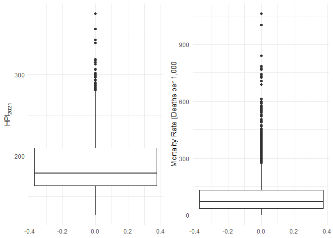
Summary Statistics of Key Numeric Variables:
| Variable | Mean | Median | SD | Min | Max |
|---|---|---|---|---|---|
| HPI 2015 | 140.88 | 136.14 | 24.76 | 85.82 | 348.52 |
| HPI 2016 | 145.87 | 140.07 | 25.17 | 90.43 | 322.69 |
| HPI 2017 | 151.83 | 144.78 | 26.31 | 97.95 | 319.03 |
| HPI 2018 | 158.83 | 151.28 | 28.06 | 104.95 | 334.27 |
| HPI 2019 | 165.68 | 157.21 | 30.07 | 110.39 | 357.13 |
| HPI 2020 | 171.50 | 162.37 | 31.38 | 115.14 | 367.03 |
| HPI 2021 | 189.67 | 178.99 | 36.41 | 127.46 | 374.60 |
| Mortality Rate | 102.08 | 70.60 | 103.19 | 0.00 | 1062.03 |
How COVID-19 Mortality Rates Compare Against $\text{HPI}_{2021}$
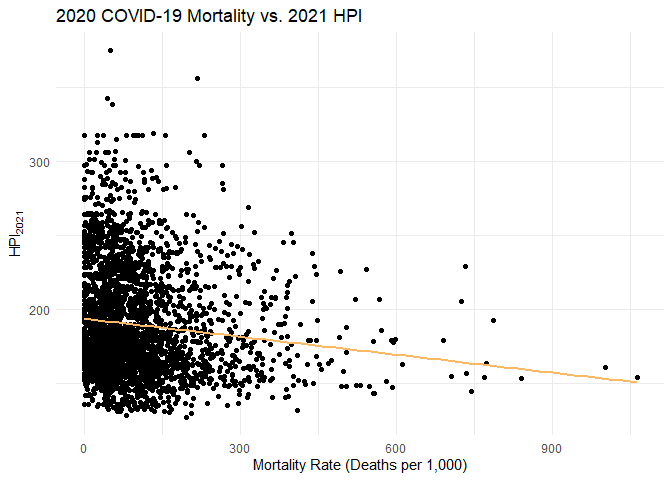
Initial trends indicate that there’s a general negative trend between mortality rate and $\text{HPI}_{2021}$.
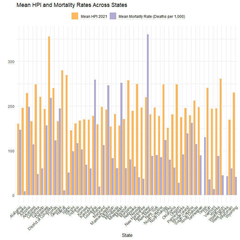
This demonstrates the variability between states’ $\text{HPI}_{2021}$ and COVID-19 mortality rates. The fact that the proportion of $\text{HPI}_{2021}$ and mortality rate varies drastically depending on state indicates that both mortality and $\text{HPI}_{2021}$ may depend on the state and state-specific policies. In econometric terms, we need to include state-specific fixed effects in our econometric model in order to further satisfy $E[\epsilon|X]=0$
Econometric Model
It is hypothesized that there are unobserved effects in the data that are dependent upon each state ($s$) such that for each county ($c$) that we wish to estimate the COVID-19 mortality effect on per-county housing prices in 2021 ($\text{HPI}_{2021}$), the error term ($\epsilon$) can thus be represented by $\epsilon_{sc}=\alpha_s+\eta_{st}$. We will remedy this issue by using a fixed effects model by including $n-1$ dummy variables for $n$ states.
Furthermore, due to the lagged effects in the model, the theoretical model incorporates some time effect $t$, where $t$ is the specified year. Including these lagged effects in the econometric model will make the estimate for the coefficient on COVID-19 mortality less biased since it will be ridden from the time-trends in HPI that occur due to the nature of time-series dependent data. Excluding the lags from model will likely lead to a biased coefficient on the estimated effect for mortality, as it would have encapsulated the effects of the lagged variables in $\eta_{sc}$ which would have otherwise been controlled for in the model Since $\text{HPI}_{2021}$ is significantly dependent upon $\text{HPI}_{2021-1},…,\text{HPI}_{2021-P}$ (as shown in A.1), where $P$ is the number of lags in the model (in this analysis we let $P=6$), then since $\delta_p > 0 \quad \forall p \in {1,…,P}$, then the coefficient for mortality will be overestimated if the lag variables are excluded from the model.
Hence, for year $t$, state $s$, and county $c$, we wish to estimate for $n$ # of states,
-
$\text{HPI}_{sct} = \beta_0+\beta_1 + \text{Mortality}_{sct-1} + \sum_{j=1}^{n-1} + \beta_{j+1}I(\text{State}_s=j) +$
$\sum_{p=1}^{6}\delta_{p} + \text{HPI}_{sct-p} + \eta_{sct}$
Where $\beta_1$ is the parameter of interest. Since we are only interested in the effect that 2020 COVID-19 mortality had on 2021 per-county housing prices, setting $t=2021$ yields a regression on a cross-sectional data set
Since we include only $n-1$ dummy variables for $n$ # of states, $X’X$ will be full rank and thus invertible. Since we control for state effects using a fixed effects model we further satisfy the assumption that $E[\eta_{sc}|X]=0$. This assumption is more reasonably satisfied with the inclusion of lagged effects on $\text{HPI}_{sct=2021}$. Since these lagged effects significantly affect the main response, $\text{HPI}_{sct=2021}$, including them in the model will isolate the estimated causal effect for $\beta_1$.
Findings
Using OLS to estimate $\beta_1$, we arrived at the following estimate (see A.2 for full model output):
| Coefficient | Estimate | Std. Error | T.Value | P.Value | 2.5 % | 97.5 % |
|---|---|---|---|---|---|---|
| Mortality Rate | -0.0031 | 0.0006105 | -5.07407 | 0.00000041 | -0.0043 | -0.0019 |
Adjusted $R^2$ = 0.9936818
Controlling for the a state-fixed effects and lagged effects on $\text{HPI}_{sct=2021}$, the estimate for $\beta_1$ was found to be highly significant and negative.
Holding all else constant, an additional COVID-19 mortality per 1,000 residents decreases the county-average 2021 housing price index by an 0.0031, on average.
Holding all else constant, we are 95% confident that an additional COVID-19 mortality per 1,000 residents decreases the 2021 county-average housing price index between 0.0043 and 0.0019, on average.
Conclusions
The conclusions following the empirical analysis align with economic theory. On average, fewer consumers in the housing market lead to an average decrease in the price on average. Controlling for all other relevant effects, the increase in per-county COVID-19 mortality implies a decrease in per-county 2021 HPI, on average. Though the housing prices over the past six years have generally risen, there is significant evidence to believe that on the county-level, 2021 HPI would have risen higher if COVID-19 mortality could have been mitigated on the county-level as well.
Limitations
Though the econometric model (1) controlled for as much as bias as possible to obtain an unbiased estimate for $\beta_1$, the model suffers from missing data in $X$. Though the NYT’s public database is one of the most up to date data bases on per-county COVID mortalities, some counties were marked as “unknown”, due to some state health department procedures. In addition, as mentioned earlier, several geographical exceptions made it impractical to measure the impact of per-county COVID-19 mortalities on housing prices for larger jurisdictions that cover multiple counties such as New York and Kansas City. In the cases where multiple counties or other non-county geographies were grouped as a single county, the fips code was dropped making it impractical to join with per-county housing price data.
Additionally, housing price indices were aggregated over the county-specific zip-codes and computed as a mean for each county. A future analysis would weight these HPIs by the population weights in each zip code. This analysis assumes each zip code is weighted equally in population.
Appendix
A.1
I determined a sufficient # of lags ($P$) for the lagged effects on $\text{HPI}_{sct=2021}$ by regressing $\text{HPI}_{sct=2021}$ on $\text{HPI}_{sct-1},…,\text{HPI}_{sct-P}$ until the last the regression coefficient, $\delta_{P}$, was no longer significant for a chosen level of significance, $\alpha$. Let $\alpha=0.1$
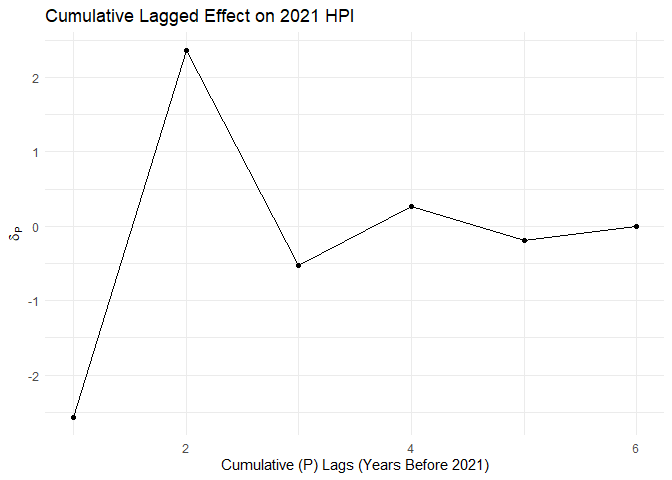
Hence, let $P=6$.
A.2
Full regression output for estimates on (1). (See also log file)
| Coefficient | Estimate | Std. Error | T.Value | P.Value | 2.5 % | 97.5 % |
|---|---|---|---|---|---|---|
| $\beta_0$ | 9.08027 | 0.6515312 | 13.93682 | 0.00000000 | 7.80279 | 10.35776 |
| Mortality Rate | -0.00310 | 0.0006105 | -5.07407 | 0.00000041 | -0.00430 | -0.00190 |
| HPI 2015 | -0.35359 | 0.0229598 | -15.40042 | 0.00000000 | -0.39861 | -0.30857 |
| HPI 2016 | -0.02682 | 0.0452753 | -0.59248 | 0.55357000 | -0.11560 | 0.06195 |
| HPI 2017 | 0.20687 | 0.0430709 | 4.80295 | 0.00000164 | 0.12242 | 0.29132 |
| HPI 2018 | -0.13237 | 0.0412066 | -3.21236 | 0.00133018 | -0.21317 | -0.05157 |
| HPI 2019 | -0.59148 | 0.0437516 | -13.51910 | 0.00000000 | -0.67727 | -0.50570 |
| HPI 2020 | 1.86692 | 0.0324828 | 57.47427 | 0.00000000 | 1.80323 | 1.93061 |
| Alaska | 0.87602 | 0.7252829 | 1.20783 | 0.22720542 | -0.54607 | 2.29811 |
| Arizona | 9.70355 | 0.8636497 | 11.23551 | 0.00000000 | 8.01015 | 11.39694 |
| Arkansas | 2.48756 | 0.4915096 | 5.06106 | 0.00000044 | 1.52384 | 3.45128 |
| California | 6.89466 | 0.6093635 | 11.31452 | 0.00000000 | 5.69985 | 8.08946 |
| Colorado | 2.87857 | 0.5502238 | 5.23163 | 0.00000018 | 1.79972 | 3.95741 |
| Delaware | 5.75894 | 1.7115600 | 3.36473 | 0.00077563 | 2.40302 | 9.11487 |
| District of Columbia | 0.44122 | 3.0003582 | 0.14705 | 0.88309895 | -5.44171 | 6.32414 |
| Florida | 4.68318 | 0.5734236 | 8.16706 | 0.00000000 | 3.55885 | 5.80752 |
| Georgia | 0.42052 | 0.4279287 | 0.98268 | 0.32584226 | -0.41854 | 1.25957 |
| Hawaii | 5.58311 | 1.4297505 | 3.90495 | 0.00009628 | 2.77974 | 8.38648 |
| Idaho | 10.65327 | 0.7255525 | 14.68297 | 0.00000000 | 9.23065 | 12.07589 |
| Illinois | 0.17282 | 0.4656942 | 0.37110 | 0.71058516 | -0.74028 | 1.08593 |
| Indiana | 0.67766 | 0.4708831 | 1.43912 | 0.15021823 | -0.24562 | 1.60094 |
| Iowa | -0.68887 | 0.4729804 | -1.45645 | 0.14537018 | -1.61627 | 0.23852 |
| Kansas | -0.08220 | 0.4611358 | -0.17825 | 0.85854226 | -0.98636 | 0.82197 |
| Kentucky | 0.40446 | 0.4493046 | 0.90018 | 0.36809361 | -0.47651 | 1.28543 |
| Louisiana | -0.76242 | 0.5327908 | -1.43100 | 0.15253188 | -1.80709 | 0.28224 |
| Maine | 0.14863 | 0.8118053 | 0.18309 | 0.85473815 | -1.44310 | 1.74037 |
| Maryland | 4.10228 | 0.7012481 | 5.84996 | 0.00000001 | 2.72731 | 5.47724 |
| Massachusetts | 2.26367 | 0.8603208 | 2.63120 | 0.00855122 | 0.57681 | 3.95054 |
| Michigan | 0.69564 | 0.4874590 | 1.42707 | 0.15366069 | -0.26014 | 1.65142 |
| Minnesota | 1.33058 | 0.4866585 | 2.73410 | 0.00629108 | 0.37636 | 2.28479 |
| Mississippi | -0.22151 | 0.4857819 | -0.45599 | 0.64842859 | -1.17400 | 0.73098 |
| Missouri | 2.29708 | 0.4503887 | 5.10021 | 0.00000036 | 1.41398 | 3.18017 |
| Montana | 9.33223 | 0.6064473 | 15.38836 | 0.00000000 | 8.14314 | 10.52131 |
| Nebraska | 0.49024 | 0.4842142 | 1.01245 | 0.31140438 | -0.45918 | 1.43966 |
| Nevada | 7.79373 | 0.8445802 | 9.22794 | 0.00000000 | 6.13773 | 9.44974 |
| New Hampshire | 1.98369 | 0.9927911 | 1.99809 | 0.04579509 | 0.03708 | 3.93029 |
| New Jersey | 3.80694 | 0.7612258 | 5.00107 | 0.00000060 | 2.31437 | 5.29951 |
| New Mexico | -0.03753 | 0.6253614 | -0.06001 | 0.95215054 | -1.26370 | 1.18864 |
| New York | 2.84983 | 0.5398307 | 5.27911 | 0.00000014 | 1.79136 | 3.90830 |
| North Carolina | 3.08102 | 0.4630017 | 6.65445 | 0.00000000 | 2.17320 | 3.98885 |
| North Dakota | 2.18345 | 0.6718277 | 3.25001 | 0.00116651 | 0.86617 | 3.50073 |
| Ohio | -0.90850 | 0.4762208 | -1.90773 | 0.05651970 | -1.84225 | 0.02524 |
| Oklahoma | 2.55833 | 0.4972734 | 5.14471 | 0.00000028 | 1.58330 | 3.53335 |
| Oregon | 5.49660 | 0.6729647 | 8.16774 | 0.00000000 | 4.17709 | 6.81611 |
| Pennsylvania | 1.16220 | 0.5061576 | 2.29612 | 0.02173633 | 0.16976 | 2.15464 |
| Rhode Island | 2.69825 | 1.3474705 | 2.00246 | 0.04532383 | 0.05621 | 5.34029 |
| South Carolina | 1.52320 | 0.5600854 | 2.71959 | 0.00657320 | 0.42502 | 2.62139 |
| South Dakota | 2.32386 | 0.5424788 | 4.28379 | 0.00001894 | 1.26020 | 3.38752 |
| Tennessee | 4.61973 | 0.4815199 | 9.59405 | 0.00000000 | 3.67559 | 5.56386 |
| Texas | 2.58799 | 0.4423724 | 5.85026 | 0.00000001 | 1.72062 | 3.45537 |
| Utah | 10.62956 | 0.6978804 | 15.23121 | 0.00000000 | 9.26120 | 11.99792 |
| Vermont | 0.94603 | 0.8657926 | 1.09268 | 0.27462088 | -0.75156 | 2.64363 |
| Virginia | 2.44825 | 0.4504892 | 5.43464 | 0.00000006 | 1.56496 | 3.33154 |
| Washington | 4.22278 | 0.6794959 | 6.21458 | 0.00000000 | 2.89047 | 5.55510 |
| West Virginia | 0.55756 | 0.5466830 | 1.01990 | 0.30785529 | -0.51434 | 1.62947 |
| Wisconsin | 0.32255 | 0.5009011 | 0.64393 | 0.51966771 | -0.65959 | 1.30468 |
| Wyoming | 4.29918 | 0.7469335 | 5.75577 | 0.00000001 | 2.83464 | 5.76372 |