Introduction
The NCAA Men’s Basketball tournament has been a well-known and highly anticipated sporting event since 1939 for not only the athletic aspects of the game, but also for the prediction of winning brackets. In the realm of sports analytics and statistical modeling, the question of replicating tournament outcomes has become an increasingly intriguing challenge. Although there are various covariates that contribute to whether a team wins or lose, we aim to utilize the Field Goal Attempts (FGA) data from the 2022 regular season to replicate the 2023 results of the tournament. Upon running a simulation of the 2023 NCAA March Madness Tournament with our model, we found that of the 358 teams, Gonzaga and Oral Roberts ended up in the final championship match. We will choose Gonzaga and Oral Roberts to follow along as we conduct a further analysis.
Methods
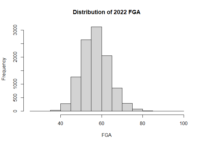
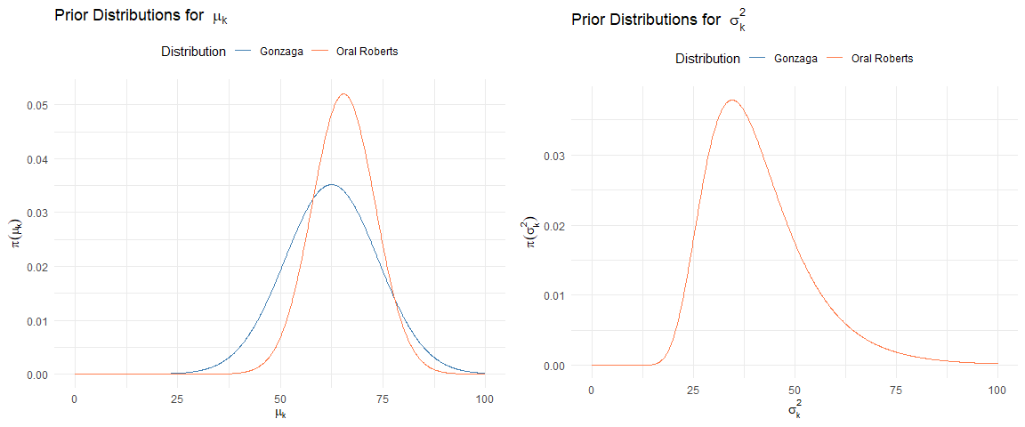
Field Goals Attempted (FGA): Upon looking at the 2022 regular season data, we observed the distribution of FGA to be approximately normal (A.0). Therefore, we will assume that the true distributions for FGA for each $k$th team is also normally distributed and use a normal distribution with mean $\mu_k$ and variance $\sigma_k^2$ as our prior distribution. Thus, to calculate FGA, we will have two unknown parameters, $\mu_k$ and $\sigma^2_k$ and will use Gibbs Sampling to approximate the following prior parameters from our 2022 regular season data:
-
$\mu_k \sim N(\lambda_k,\tau_k); \quad \mu_\text{Gonzaga} \sim N$(62.48, 11.33$^2); \quad \mu_\text{Oral Roberts} \sim N$(65.46, 7.67$^2)$
-
$\sigma^2_{k} \sim \text{InvGam}(\gamma,\phi) \quad \forall k; \quad \sigma^2 \sim \text{InvGam}(\gamma$=11.79,$\phi$=441.6)
Then our likelihood would be $\text{FGA}_{ki} \sim N(\mu_k,\sigma^2_{k})$ and our posterior distribution is then the joint posterior, $(\mu_k, \sigma^2_{k})$. The subscript $i$ denotes the $i$th observation (FGA) for the $k$th team. (See A.3 for plot code.)
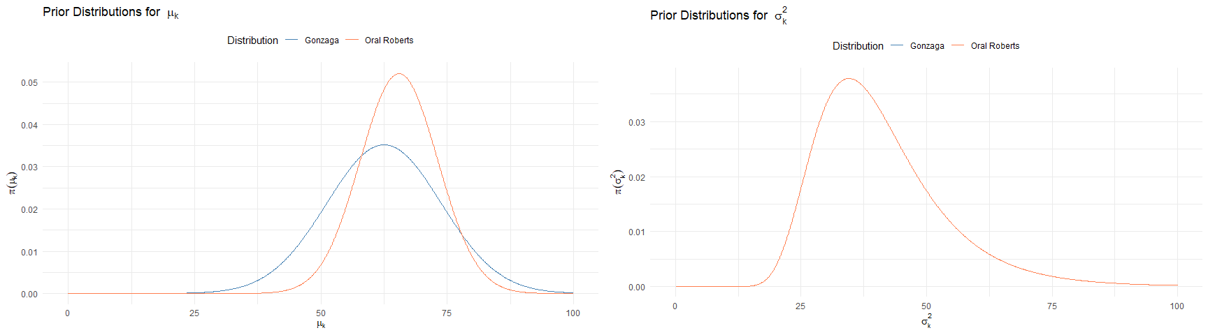
Prior parameters were chosen such that for each $k$th team, $\mu_k$ was the mean of $\text{FGA}_{ik}$ from the NCAA 2022 season and $\sigma_k$ was chosen as the range of the $\text{FGA}_{ik}$ divided by 3–dividing by 6 would approximate the standard deviation given that the range is an unbiased estimator for the 99.7% interquartile range, thus dividing by 3 adds more uncertainty about our belief and less influence from the 2022 season. $\gamma_k$ and $\phi_k$ were chosen as a generic prior using a method of moments from data from the 2022 season to select unbiased estimators for the variance of FGA across all teams A.4.
Field Goal Percentage (FGP): FGP is a proportion calculated from FGA divided by FGM. Utilizing the 2022 regular season data, we modeled our prior distribution below:$\text{FGP}_{k} \sim Beta(\alpha_k,\beta_k)$
For each game $g$ and team $k$, our likelihood is $X_{gki} \sim Binom(\text{FGP}_{k})$, as we are modeling the idea that players either make the basket ($X_{gki}$) or do not. Then, as we have a binomial likelihood and a beta conjugate prior, we have a beta posterior distribution as follows: $\text{FGP}_{k}|Data_k \sim Beta(\alpha_k,\beta_k)$. Due to our questions of interest and compactness, we will not explore the posterior distribution for FGP in depth here and will refer to the appendix (A.2)
Priors:
$\text{FGP}_\text{Gonzaga}\sim \text{Beta}(1.12, 1); \quad$ $\text{FGP}_\text{Oral Roberts}\sim \text{Beta}(0.8290895, 1)$
For each $k$th team the posterior will be: $\text{FGP}_k|\text{Data}_k\sim \text{Beta}(\alpha’,\beta’);$ $\alpha’=\sum_{g=1}^{n_k}\sum_{i=1}^{n_{gki}}x_{gki}+\alpha_k;$ $\beta’=\sum_{g=1}^{n_k}\sum_{i=1}^{n_{gki}}1-\sum_{g=1}^{n_k}\sum_{i=1}^{n_{gki}}x_{gki}+\beta_k$ where $n_k$ is the # of games for team $k$, and $n_{gki}$ is the number of shots team $k$ attempts in game $g$.
$\text{FGP}_\text{Gonzaga}|\text{Data}_\text{Gonzaga}\sim \text{Beta}(1026.12, 939)$ $\text{FGP}_\text{Oral Roberts}|\text{Data}_\text{Oral Roberts}\sim \text{Beta}(1026.12, 939)$
Field Goals Made (FGM)
Research Question: Given our observations from the 2022 season, can we calculate overall Field Goals Made (FGM) and can we use FGM to predict which team would win in a match?
If $\zeta_k$ is the true population mean of $\text{FGM}_{ik}$, We will estimate the following posterior distribution: $\zeta_{k}|\text{Data}_k$, where the random variable $\text{FGM}_{ik}=\text{FGA}_{ik} \times \text{FGP}_{ik}$
Using this posterior, we wish to approximate, $\text{FGM}_{k} | {Data}_k > \text{FGM}_{l} {|Data}_l, \text{where } \textit{k } \text{and } \textit{l } \text{are teams,} \forall k \neq {l}$ to determine the probability team $k$ will score more field goals than team $l$. Thus, $\text{FGM}_{k} {|Data}_k > \text{FGM}_{l} {|Data}_l \sim \text{Bernoulli}(p_{kl})$
Summary Statistics of Key Variables for the 2023 Season (Aggregated accross all teams)
| Variable | Mean | Median | SD | Min | Max |
|---|---|---|---|---|---|
| FGP | 0.4424 | 0.4423 | 0.0719 | 0.1786 | 0.7193 |
| FGA | 57.2391 | 57.0000 | 6.8474 | 26.0000 | 91.0000 |
| FGM | 25.2510 | 25.0000 | 4.7402 | 9.0000 | 47.0000 |
We obtained data for FGA and FGM for each team through publicly available data sets (see Data Sources). See “Set Up” in the appendix to see how we wrangled the data.
Results
Posterior Distributions for FGA for Each $k$th Team:
$\mu_k|\text{Data}_k,\sigma^2_k \sim N(\lambda’_k, (\tau^2)_k’) \quad \lambda’_k = \frac{\tau_k^2(\sum_{i=1}^{n_k}x_{ki})+\sigma_k^2\lambda_k}{\tau_k^2} \quad (\tau^2_k)’=\frac{\sigma_k^2\tau_k^2}{\tau_k^2n_k+\sigma_k^2}$
$\sigma^2_k|\text{Data}_k,\mu_k ~ \text{InvGamma}(\gamma_k’,\phi_k’) \quad \gamma_k’=\gamma_k+\frac{n_k}{2} \quad \phi_k’=\frac{\phi_k\sum_{i=1}^{n_k}(x_{ik}-\mu_k)}{2}$
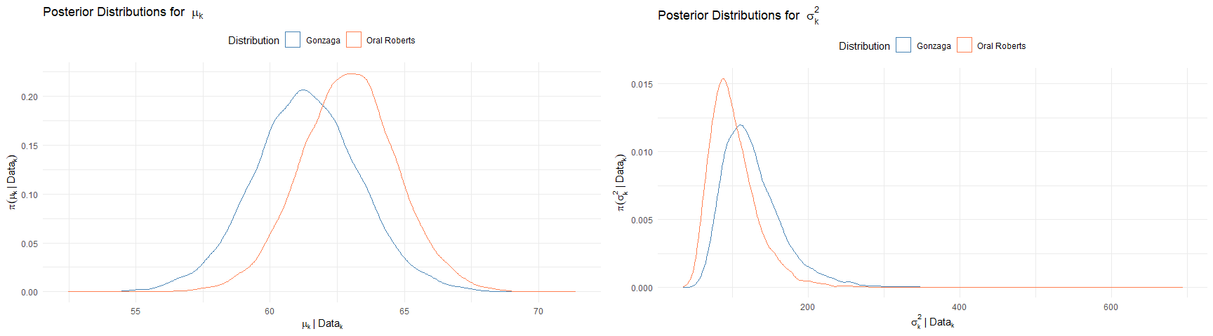
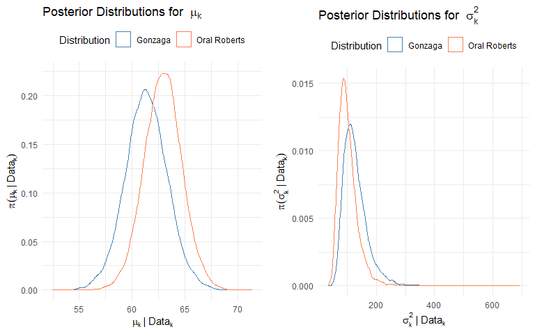
Joint Distribution of $(\mu_k, \sigma^2_k)$ Approximated with Gibbs Sampling (See A.6 for plot code):
| Parameter | Gonzaga | Oral Roberts |
|---|---|---|
| Expected Value for $\mu$ | 61.3506974 | 62.9155502 |
| Variance for $\mu$ | 3.9418405 | 3.2074749 |
| Expected Value for $\sigma^2$ | 127.0707504 | 102.1374316 |
| Variance for $\sigma^2$ | 1664.3040285 | 1096.8885862 |
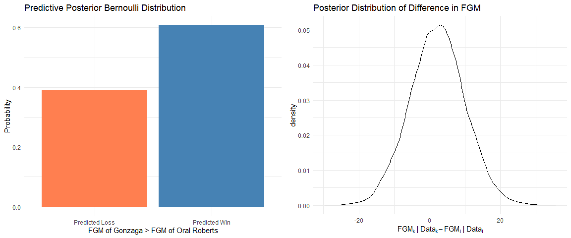
Posterior Predictive Distribution on FGM (See A.7 for plot code):
$\text{FGM}_{k}|\text{Data}_k > \text{FGM}_l|\text{Data}_k \sim \text{Bernoulli}(p_{kl}); p_{\text{Gonzaga},\text{Oral Roberts}} = 0.629$
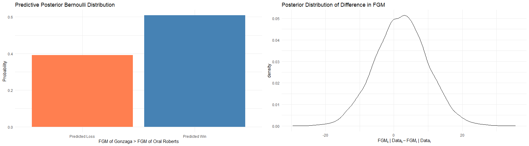
Our estimated posterior predictive variance using Monte Carlo Approximation were 2.16 and 61.49 (respectively)
95% Credible Interval for Difference in FGM: Given our data and prior knowledge, the there is a 95% probability that the difference in FGM between Gonzaga and Oral Roberts will be between -13.27 and 17.63.
Conclusions
Through deriving a posterior predictive distribution on the difference in the number FGM for any two teams we created a model for predicting the probability that one team will score more field goals (and thus have a higher chance of winning) over their opponent. However, we discovered that virtually all matchups had significant overlaps such that any 95% credible interval showed that using FGM as a metric alone, it was just as probable for the other team to score more FG than what our bernoulli model predicts. The Gonzaga-Oral Roberts matchup is just one notable example. One of the greatest limitations in this model is its failures to account for the opponent’s defense. There are certainly other confounders that can be adjusted for. However, this model shows that, at least for Oral Roberts and Gonzaga, the prior estimate of 2022 may be somewhat of an accurate prediction of 2023 FGA. With reduced variability, the posterior model shows similar FGA measures to the 2022 prior estimates.
Appendix
Data Sources
-
2022 and 2023 NCAA season data was obtained through Kaggle: https://www.kaggle.com/competitions/march-machine-learning-mania-2023. We obtained FGA and FGM data for each team through the data sets located here.
-
2023 Tournament Data was obtained through Kaggle: https://www.kaggle.com/datasets/nishaanamin/march-madness-data?select=2023+Game+Data.csv. We used this data set to set up the a tournament simulation.
Set up
library(tidyverse)
library(invgamma)
library(ggplot2)
library(gridExtra)

set.seed(12142023)

data_dir = "march-machine-learning-mania-2023/"

season_results = read_csv(str_c(data_dir, "MRegularSeasonDetailedResults.csv"))
teams = read_csv(str_c(data_dir, "MTeams.csv"))
tourney_results = read_csv("2023 Game Data.csv")

transform_data = function(t){
  t %>% pivot_longer(cols=c(WTeamID, LTeamID), names_to="WL", values_to = "TeamID") %>%
  select(TeamID, WL, WScore, LScore, WFGM, WFGA, LFGM, LFGA) %>%
  left_join(teams %>% select(TeamID, TeamName)) %>%
  pivot_longer(cols=c(WScore, LScore), values_to = "Score", names_to = "WLScore") %>%
  pivot_longer(cols=c(WFGM, LFGM), values_to="FGM", names_to = "WLFGM") %>%
  pivot_longer(cols=c(WFGA, LFGA), values_to="FGA", names_to = "WLFGA") %>%
  mutate(WL = sapply(WL, function(x)substr(x,1,1)),
         WLScore = sapply(WLScore, function(x)substr(x,1,1)),
         WLFGM = sapply(WLFGM, function(x)substr(x,1,1)),
         WLFGA = sapply(WLFGA, function(x)substr(x,1,1))
  ) %>% rowwise() %>%
  filter(all(c(WL, WLScore, WLFGM, WLFGA) ==
               first(c(WL, WLScore, WLFGM, WLFGA)))) %>%
  select(TeamID, WL, TeamName, Score, FGM, FGA)
}

#2022 Season
season.2022 <- season_results %>%
  filter(Season %in% 2022)

season.2022 <- transform_data(season.2022)

season.2022 %>% mutate(
    FGP = FGM/FGA
  ) -> season.2022
Calculate priors
calculate_prior_fgp = function(p, beta=1){
  #Returns alpha for a Beta(alpha, beta) such that alpha/(alpha+beta) =
  #p (expected value)
  return(p*beta/(1-p))
}

#Calculate priors for the field goal percentage ~ Beta(alpha, beta)
#and for the field goal attempts ~ N(mu, sigma^2)
season.2022 %>% group_by(TeamID) %>%
  summarize(
    fgp.alpha.prior = calculate_prior_fgp(mean(FGP)),
    fgp.beta.prior = 1,
    fga.lambda.prior = mean(FGA),
    fga.tau.prior = (max(FGA)-min(FGA))/3
  ) %>% ungroup() -> season.2022.priors

variances = season.2022 %>% group_by(TeamID) %>%
  summarize(
    variances = var(FGA)
  )
#Method of Moments https://arxiv.org/pdf/1605.01019.pdf
#To create a generic prior for all k teams
season.2022.priors$fga.gamma.prior = mean(variances$variances)^2/
  var(variances$variances)+2
season.2022.priors$fga.phi.prior =
  mean(variances$variances)*(mean(variances$variances)^2/
                                             var(variances$variances)+1)

#2023 Season we want to model
season.2023 <- season_results %>%
  filter(Season %in% 2023)

season.2023 <- transform_data(season.2023)
Calculation of Beta Posterior for each $k$th Team
#Calculate posteriors for FGP for the 2023 season
season.2023.posteriors = season.2023 %>%
  left_join(season.2022.priors, by=join_by(TeamID)) %>%
  group_by(TeamID) %>%
  summarize (
    fgp.alpha.posterior = sum(FGM)+first(fgp.alpha.prior),
    fgp.beta.posterior = sum(FGA)-sum(FGM)+first(fgp.beta.prior)
  )
Gibbs Sampling to Approximate Joint Distribution $(\mu_k, \sigma^2_k)$
#Gibbs Sampling Method to Define Posterior
posterior.matrix = as.matrix(
  season.2023.posteriors[c("fga.lambda.prior", "fga.tau.prior",
                           "fga.gamma.prior", "fga.phi.prior")])

iterations = 10000

#Matrices to store posterior distributions
posterior.normal.matrix = matrix(ncol=iterations, nrow=nrow(posterior.matrix))
posterior.invgamma.matrix = matrix(ncol=iterations, nrow=nrow(posterior.matrix))

#Calculate the Normal posterior distribution for each ith team via Gibbs sampling
for(i in 1:nrow(posterior.matrix)){
  ith_team = posterior.matrix[i,]
  data_i = season.2023[season.2023$TeamID ==
                         as.numeric(season.2023.posteriors[i,"TeamID"]), "FGA"] %>%
    unlist()

  #Gibbs sampling algorithm
  burn = 100
  iters <- iterations + burn
  mu.save <- rep(0, iters)
  mu.save <- ith_team["fga.lambda.prior"]
  sigma2.save <- rep(0, iters)
  sigma2 = ith_team["fga.phi.prior"]/(ith_team["fga.gamma.prior"]-1)
  sigma2.save[1] = sigma2

  lambda = ith_team["fga.lambda.prior"]
  tau = ith_team["fga.tau.prior"]
  gamma = ith_team["fga.gamma.prior"]
  phi = ith_team["fga.phi.prior"]
  n = length(data_i)

  if(any(is.na(ith_team))){
    posterior.normal.matrix[i,] = rep(NA_real_, iterations)
    posterior.invgamma.matrix[i,] = rep(NA_real_, iterations)
  } else {
    for(t in 2:iters){
      #Full conditional of mu
      lambda.p <- (tau^2*sum(data_i) + sigma2*lambda)/(tau^2*n + sigma2)
      tau2.p <- sigma2*tau^2/(tau^2*n + sigma2)

      #New value of mu
      mu <- rnorm(1, lambda.p, sqrt(tau2.p))
      mu.save[t] <- mu

      #Full conditional of sigma2
      gamma.p <- gamma + length(data)/2
      phi.p <- phi + sum((data_i - mu)^2)/2

      #New value of sigma2
      sigma2 <- rinvgamma(1, gamma.p, phi.p)
      sigma2.save[t] <- sigma2
    }

    posterior.normal.matrix[i,] = mu.save[-(1:burn)]
    posterior.invgamma.matrix[i,] = sigma2.save[-(1:burn)]
  }

  #print(i)

}
Posterior Predictive Computations to Approximate FGM
season.2023.posteriors$fga.mu.posterior = rowMeans(posterior.normal.matrix)
season.2023.posteriors$fga.sigma.posterior =
  sqrt(rowMeans(posterior.invgamma.matrix))

season.2023.posteriors %>%
  filter(!is.na(fga.mu.posterior)) -> season.2023.posteriors

#Monte Carlo Simulation to Simulate FGM
posterior.fgm.matrix =
  matrix(ncol=iterations, nrow=nrow(season.2023.posteriors))
for(i in 1:nrow(season.2023.posteriors)){
  #Randomly sample from p from the posterior beta distribution on
  #Field Goal Percentage
  p = rbeta(iterations,
            as.numeric(season.2023.posteriors[i, "fgp.alpha.posterior"]),
            as.numeric(season.2023.posteriors[i, "fgp.beta.posterior"]))
  #Calculate distribution of mean FGM by multiplying p by a random sample of FGA by
  #team i
  #Randomly sample from the joint distribution of mu and sigma^2
  f = rnorm(iterations, posterior.normal.matrix[i,],
            sqrt(posterior.invgamma.matrix[i,]))

  posterior.fgm.matrix[i,] = p*f
}
A.0
The distribution of FGA is approximately Normal
hist(season.2022$FGA, main="Distribution of 2022 FGA", xlab="FGA")
A.1
Simulation of NCAA Tournament Using our Predictive Posterior Bernoulli Model
Clean Tournament Data
tourney_results[c("SEED", "TEAM...3")] %>%
  setNames(c("Seed", "TeamName")) -> tourney_results
clean_team_names = function(t){
  t$TeamName = sapply(t$TeamName, function(x){
    x = x %>% str_replace("[.]", "")
    x = x %>% str_replace("Florida", "FL")
    if(x == "Saint Mary's")x = "St Mary's CA"
    if(x == "College of Charleston")x = "Col Charleston"
    if(x == "Louisiana Lafayette")x = "Lafayette"
    if(x == "Fairleigh Dickinson")x = "F Dickinson"
    if(x == "Northern Kentucky")x = "N Kentucky"
    if(x == "Southeast Missouri St")x = "SE Missouri St"
    if(x == "Texas A&M Corpus Chris")x = "TAM C. Christi"
    if(x == "Texas Southern")x = "TX Southern"
    if(x == "Montana St")x = "Montana St"
    if(x == "Kennesaw St")x = "Kennesaw"
    if(x == "Kent St")x = "Kent"
    if(x == "North Carolina St")x = "NC State"
    return(x)
  })
  return(t)
}
tourney_results = clean_team_names(tourney_results)

tourney_results %>%
  left_join(teams[c("TeamID", "TeamName")]) -> tourney_results

#Omit the first four
tourney_results %>%
  filter(!TeamName %in% c("TX Southern", "Nevada",
                          "Mississippi St", "SE Missouri St")) %>%
  distinct() -> tourney_results

tourney_results$Region = rep(c("E", "S", "W", "M"), each=2, times=8)
Simulation
#2023 Tournament Simulation

regions = c("E", "S", "W", "M")
tourney_results %>% group_by(Region) %>%
  mutate(
    Order = rep(LETTERS[1:(n()/2)], each=2)
  ) -> tourney_results

matchups = tibble()

compare_teams = function(k, l, alpha=0.25){
  k = which(season.2023.posteriors$TeamID == k)
  l = which(season.2023.posteriors$TeamID == l)
  list(
    p = mean(posterior.fgm.matrix[k,] > posterior.fgm.matrix[l,]),
    q = quantile(posterior.fgm.matrix[k,] - posterior.fgm.matrix[l,], alpha)
  )
}

tourney_results$Round = 1

for(round in 1:4){
 for(region in regions){
    t = tourney_results
    if(round > 1)t = matchups

    if(round < 5){
      #These are all the regional matches
      region.subset = t %>%
        filter(Region == region & Round == round)
    }

    region.subset$p = NA_real_
    region.subset$alpha.probability = NA_real_
    region.subset$Round = round+1
    if(round > 1){
      half = region.subset$Order[1:(length(region.subset$Order)/2)]
      region.subset$Order = c(half, rev(half))

      matchups[matchups$Region == region & matchups$Round == round,
               ]$Order =c(half, rev(half))
    }


    region.subset %>%
      arrange(Order) -> region.subset

    #Loop through every game
    i = 1
    while(i < nrow(region.subset)){
      p = compare_teams(region.subset[i,]$TeamID,
                        region.subset[i+1,]$TeamID)[["p"]]
      #Predictive probability distribution is a Bernoulli Distribution
      if(p > (1-p)){
        region.subset[i,]$p = p
        region.subset[i,]$alpha.probability =
          compare_teams(region.subset[i,]$TeamID,
                region.subset[i+1,]$TeamID)[["q"]] %>% as.vector() > 0
        matchups = rbind(matchups, region.subset[i,])
      } else {
        region.subset[i+1,]$p = 1-p
        region.subset[i+1,]$alpha.probability =
          compare_teams(region.subset[i+1,]$TeamID,
                region.subset[i,]$TeamID)[["q"]] %>% as.vector() > 0
        matchups = rbind(matchups, region.subset[i+1,])
      }
      i = i + 2
    }
  }
}

#Final Four and Championship
for(round in 5:6){
  t.subset = matchups %>%
    filter(Round == round)
  t.subset$Round = round+1

  #Loop through every game
  i = 1
  while(i < nrow(t.subset)){
    p = compare_teams(t.subset[i,]$TeamID,
                      t.subset[i+1,]$TeamID)[["p"]]
    #Predictive probability distribution is a Bernoulli Distribution
    if(p > (1-p)){
      t.subset[i,]$p = p
      t.subset[i,]$alpha.probability = compare_teams(t.subset[i,]$TeamID,
              t.subset[i+1,]$TeamID)[["q"]] %>% as.vector() > 0
      matchups = rbind(matchups, t.subset[i,])
    } else {
      t.subset[i+1,]$p = 1-p
      t.subset[i+1,]$alpha.probability = compare_teams(t.subset[i+1,]$TeamID,
              t.subset[i,]$TeamID)[["q"]] %>% as.vector() > 0
      matchups = rbind(matchups, t.subset[i+1,])
    }
    i = i + 2
  }
}
The column p indicates the predictive posterior probability of how likely that team was to make more field goals than their opposing team in the previous round.
First Round Match-ups
| Seed | TeamName | Region |
|---|---|---|
| 1 | Alabama | E |
| 16 | TAM C. Christi | E |
| 1 | Purdue | S |
| 16 | F Dickinson | S |
| 1 | Houston | W |
| 16 | N Kentucky | W |
| 1 | Kansas | M |
| 16 | Howard | M |
| 2 | Arizona | E |
| 15 | Princeton | E |
| 2 | Marquette | S |
| 15 | Vermont | S |
| 2 | Texas | W |
| 15 | Colgate | W |
| 2 | UCLA | M |
| 15 | UNC Asheville | M |
| 3 | Baylor | E |
| 14 | UC Santa Barbara | E |
| 3 | Kansas St | S |
| 14 | Montana St | S |
| 3 | Xavier | W |
| 14 | Kennesaw | W |
| 3 | Gonzaga | M |
| 14 | Grand Canyon | M |
| 4 | Virginia | E |
| 13 | Furman | E |
| 4 | Tennessee | S |
| 13 | Lafayette | S |
| 4 | Indiana | W |
| 13 | Kent | W |
| 4 | Connecticut | M |
| 13 | Iona | M |
| 5 | San Diego St | E |
| 12 | Col Charleston | E |
| 5 | Duke | S |
| 12 | Oral Roberts | S |
| 5 | Miami FL | W |
| 12 | Drake | W |
| 5 | St Mary’s CA | M |
| 12 | VCU | M |
| 6 | Creighton | E |
| 11 | NC State | E |
| 6 | Kentucky | S |
| 11 | Providence | S |
| 6 | Iowa St | W |
| 11 | Pittsburgh | W |
| 6 | TCU | M |
| 11 | Arizona St | M |
| 7 | Missouri | E |
| 10 | Utah St | E |
| 7 | Michigan St | S |
| 10 | USC | S |
| 7 | Texas A&M | W |
| 10 | Penn St | W |
| 7 | Northwestern | M |
| 10 | Boise St | M |
| 8 | Maryland | E |
| 9 | West Virginia | E |
| 8 | Memphis | S |
| 9 | FL Atlantic | S |
| 8 | Iowa | W |
| 9 | Auburn | W |
| 8 | Arkansas | M |
| 9 | Illinois | M |
Second Round Match-ups
matchups %>%
  select(Seed, TeamName, Region, p, Round, Order) %>%
  arrange(Round, Order) %>%
  select(-Order) -> matchups

matchups %>%
  filter(Round == 2) %>%
  select(-Round) %>%
  knitr::kable()
| Seed | TeamName | Region | p |
|---|---|---|---|
| 1 | Alabama | E | 0.5463 |
| 9 | West Virginia | E | 0.5741 |
| 16 | F Dickinson | S | 0.6319 |
| 8 | Memphis | S | 0.5395 |
| 1 | Houston | W | 0.6940 |
| 8 | Iowa | W | 0.6611 |
| 1 | Kansas | M | 0.5793 |
| 8 | Arkansas | M | 0.5287 |
| 2 | Arizona | E | 0.6650 |
| 7 | Missouri | E | 0.5963 |
| 2 | Marquette | S | 0.7010 |
| 10 | USC | S | 0.5102 |
| 15 | Colgate | W | 0.5908 |
| 10 | Penn St | W | 0.6472 |
| 2 | UCLA | M | 0.6667 |
| 10 | Boise St | M | 0.6250 |
| 14 | UC Santa Barbara | E | 0.5334 |
| 11 | NC State | E | 0.5978 |
| 3 | Kansas St | S | 0.6445 |
| 6 | Kentucky | S | 0.5014 |
| 3 | Xavier | W | 0.7242 |
| 11 | Pittsburgh | W | 0.5383 |
| 3 | Gonzaga | M | 0.8343 |
| 6 | TCU | M | 0.6458 |
| 13 | Furman | E | 0.7374 |
| 12 | Col Charleston | E | 0.6592 |
| 4 | Tennessee | S | 0.7020 |
| 12 | Oral Roberts | S | 0.7232 |
| 4 | Indiana | W | 0.5917 |
| 5 | Miami FL | W | 0.6338 |
| 13 | Iona | M | 0.5234 |
| 5 | St Mary’s CA | M | 0.5445 |
Sweet 16
matchups %>%
  filter(Round == 3) %>%
  select(-Round) %>%
  knitr::kable()
| Seed | TeamName | Region | p |
|---|---|---|---|
| 1 | Alabama | E | 0.6000 |
| 13 | Furman | E | 0.5296 |
| 8 | Memphis | S | 0.5561 |
| 12 | Oral Roberts | S | 0.7526 |
| 8 | Iowa | W | 0.5611 |
| 5 | Miami FL | W | 0.5291 |
| 1 | Kansas | M | 0.5290 |
| 13 | Iona | M | 0.6243 |
| 2 | Arizona | E | 0.5554 |
| 11 | NC State | E | 0.6550 |
| 2 | Marquette | S | 0.7107 |
| 6 | Kentucky | S | 0.5815 |
| 15 | Colgate | W | 0.7102 |
| 3 | Xavier | W | 0.7134 |
| 2 | UCLA | M | 0.6438 |
| 3 | Gonzaga | M | 0.7171 |
Elite 8
matchups %>%
  filter(Round == 4) %>%
  select(-Round) %>%
  knitr::kable()
| Seed | TeamName | Region | p |
|---|---|---|---|
| 13 | Furman | E | 0.5116 |
| 2 | Arizona | E | 0.5208 |
| 12 | Oral Roberts | S | 0.5673 |
| 2 | Marquette | S | 0.6179 |
| 5 | Miami FL | W | 0.5212 |
| 3 | Xavier | W | 0.5259 |
| 13 | Iona | M | 0.5220 |
| 3 | Gonzaga | M | 0.7076 |
Final Four
matchups %>%
  filter(Round == 5) %>%
  select(-Round) %>%
  knitr::kable()
| Seed | TeamName | Region | p |
|---|---|---|---|
| 2 | Arizona | E | 0.5805 |
| 12 | Oral Roberts | S | 0.5150 |
| 3 | Xavier | W | 0.5683 |
| 3 | Gonzaga | M | 0.6920 |
Championship
matchups %>%
  filter(Round == 6) %>%
  select(-Round) %>%
  knitr::kable()
| Seed | TeamName | Region | p |
|---|---|---|---|
| 12 | Oral Roberts | S | 0.5272 |
| 3 | Gonzaga | M | 0.5959 |
Champion
matchups %>%
  filter(Round == 7) %>%
  select(-Round) %>%
  knitr::kable()
| Seed | TeamName | Region | p |
|---|---|---|---|
| 3 | Gonzaga | M | 0.6083 |
A.2
Prior distribution for FGP
k = 1211 #Gonzaga
l = 1331 #Oral Roberts

k.alpha = season.2022.priors %>%
  filter(TeamID == k) %>% pull(fgp.alpha.prior)
k.beta = season.2022.priors %>%
  filter(TeamID == k) %>% pull(fgp.beta.prior)

l.alpha = season.2022.priors %>%
  filter(TeamID == l) %>% pull(fgp.alpha.prior)
l.beta = season.2022.priors %>%
  filter(TeamID == l) %>% pull(fgp.beta.prior)

ggplot(data = data.frame(x = c(0, 1)), aes(x)) +
  stat_function(fun = dbeta, n = 1001,
                args = list(shape1 = k.alpha, shape2 = k.beta),
                aes(color = "Gonzaga"),
                show.legend=T) +
  stat_function(fun = dbeta, n = 1001,
                args = list(shape1 = l.alpha, shape2 =l.beta),
                aes(color = "Oral Roberts"), show.legend=T) +
  ylab(expression(pi(FGP[k]))) +
  xlab(expression(FGP[k])) +
  ggtitle("Prior Distributions") +
  theme_minimal() +
  labs(color = "Distribution") +
  scale_color_manual(
    values = c("Gonzaga" = "steelblue", "Oral Roberts" = "coral")) +
  theme(legend.position = "top")
Prior parameters were chosen such that for each $k$th team, $\beta_k$ was chosen as 1 to reflect our uncertainty and $\alpha_k$ was chosen such that $\frac{\alpha_k}{\alpha_k+\beta_k}=\hat{p}$ where $\hat{p}$ was chosen as the mean of $\text{FGP}_{ik}$ from the 2022 NCAA season.
$\text{FGP}_\text{Gonzaga}\sim \text{Beta}$(1026.1155142, 939) $\quad \text{FGP}_\text{Oral Roberts}\sim \text{Beta}$(1026.1155142, 939)
Posterior Distribution
$\text{FGP}_k|\text{Data}_{k} \sim \text{Beta}(\alpha_k, \beta_k) \quad \forall k \in \text{Teams}$
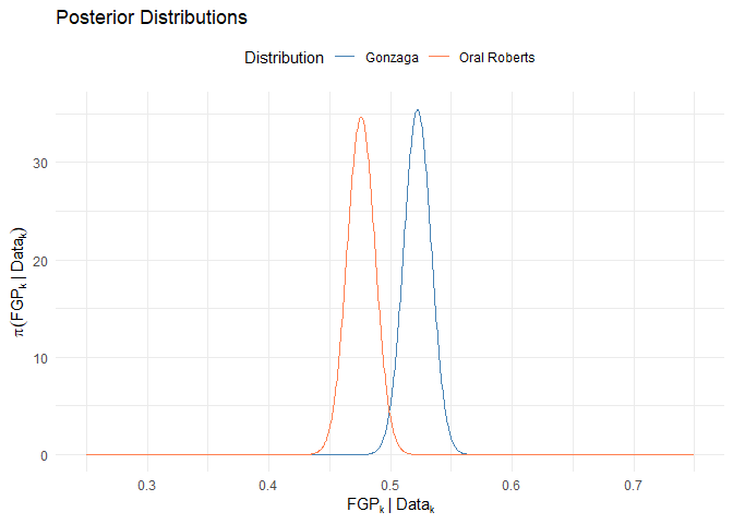
We estimated the following the posterior distributions for their Field Goal Percentage:
$\text{FGP}_\text{Gonzaga}|\text{Data}_\text{Gonzaga} \sim \text{Beta}(1026.116, 939)$
$\text{FGP}_\text{Oral Roberts}|\text{Data}_\text{Oral Roberts} \sim \text{Beta}(896.829, 988)$
Hence,
$E(\text{FGP}_\text{Gonzaga}|\text{Data}_\text{Gonzaga})=0.522$
$E(\text{FGP}_\text{Oral Roberts}|\text{Data}_\text{Oral Roberts})=0.476$
$V(\text{FGP}_\text{Gonzaga}|\text{Data}_\text{Gonzaga})$=1.2690439^{-4}
$V(\text{FGP}_\text{Oral Roberts}|\text{Data}_\text{Oral Roberts})$=1.3225751^{-4}
A.3
Prior Distribution for FGA
k = 1211 #Gonzaga
l = 1331 #Oral Roberts

k.lambda = season.2022.priors %>%
  filter(TeamID == k) %>% pull(fga.lambda.prior)
k.tau = season.2022.priors %>%
  filter(TeamID == k) %>% pull(fga.tau.prior)
k.gamma = season.2022.priors %>%
  filter(TeamID == k) %>% pull(fga.gamma.prior)
k.phi = season.2022.priors %>%
  filter(TeamID == k) %>% pull(fga.phi.prior)

l.lambda = season.2022.priors %>%
  filter(TeamID == l) %>% pull(fga.lambda.prior)
l.tau = season.2022.priors %>%
  filter(TeamID == l) %>% pull(fga.tau.prior)
l.gamma = season.2022.priors %>%
  filter(TeamID == l) %>% pull(fga.gamma.prior)
l.phi = season.2022.priors %>%
  filter(TeamID == l) %>% pull(fga.phi.prior)

mu.plot=ggplot(data = data.frame(x = c(0, 100)), aes(x)) +
  stat_function(fun = dnorm, n = 1001,
                args = list(mean = k.lambda, sd = k.tau),
                aes(color = "Gonzaga"),
                show.legend=T) +
  stat_function(fun = dnorm, n = 1001,
                args = list(mean = l.lambda, sd = l.tau),
                aes(color = "Oral Roberts"),
                show.legend=T)+
  ylab(expression(pi(mu[k]))) +
  xlab(expression(mu[k])) +
  ggtitle("Prior Distributions for "~mu[k]) +
  theme_minimal() +
  labs(color = "Distribution") +
  scale_color_manual(
    values = c("Gonzaga" = "steelblue", "Oral Roberts" = "coral")) +
  theme(legend.position = "top")

sigma2.plot = ggplot(data = data.frame(x = c(0, 100)), aes(x)) +
stat_function(fun = dinvgamma, n = 1001,
                args = list(shape = k.gamma, rate = k.phi),
                aes(color = "Gonzaga"),
                show.legend=T) +
  stat_function(fun = dinvgamma, n = 1001,
                args = list(shape = l.gamma, rate = l.phi),
                aes(color = "Oral Roberts"),
                show.legend=T) +
  ylab(expression(pi(sigma[k]^2))) +
  xlab(expression(sigma[k]^2)) +
  ggtitle("Prior Distributions for "~sigma[k]^2) +
  theme_minimal() +
  labs(color = "Distribution") +
  scale_color_manual(
    values = c("Gonzaga" = "steelblue", "Oral Roberts" = "coral")) +
  theme(legend.position = "top")

grid.arrange(mu.plot, sigma2.plot, ncol=2)
A.4
A. Llera, C. F. Beckmann., “Estimating an Inverse Gamma Distribution” (https://arxiv.org/pdf/1605.01019.pdf)
A.5
Posterior Distribution for FGP
k = 1211 #Gonzaga
l = 1331 #Oral Roberts

k.alpha = season.2023.posteriors %>%
  filter(TeamID == k) %>% pull(fgp.alpha.posterior)
k.beta = season.2023.posteriors %>%
  filter(TeamID == k) %>% pull(fgp.beta.posterior)

l.alpha = season.2023.posteriors %>%
  filter(TeamID == l) %>% pull(fgp.alpha.posterior)
l.beta = season.2023.posteriors %>%
  filter(TeamID == l) %>% pull(fgp.beta.posterior)

ggplot(data = data.frame(x = c(0.25, 0.75)), aes(x)) +
  stat_function(fun = dbeta, n = 1001,
                args = list(shape1 = k.alpha, shape2 = k.beta),
                aes(color = "Gonzaga"),
                show.legend=T) +
  stat_function(fun = dbeta, n = 1001,
                args = list(shape1 = l.alpha, shape2 =l.beta),
                aes(color = "Oral Roberts"), show.legend=T) +
  ylab(expression(pi(FGP[k]~"|"~Data[k]))) +
  xlab(expression(FGP[k]~"|"~Data[k])) +
  ggtitle("Posterior Distributions") +
  theme_minimal() +
  labs(color = "Distribution") +
  scale_color_manual(
    values = c("Gonzaga" = "steelblue", "Oral Roberts" = "coral")) +
  theme(legend.position = "top")

A.6
Joint Posterior Distribution for FGA Approximated using Gibbs Sampling
k = 1211 #Gonzaga
l = 1331 #Oral Roberts

k = which(season.2023.posteriors$TeamID == k)
l = which(season.2023.posteriors$TeamID == l)

k.mu = posterior.normal.matrix[k,]
k.sigma2 = posterior.invgamma.matrix[k,]

l.mu = posterior.normal.matrix[l,]
l.sigma2 = posterior.invgamma.matrix[l,]

mu.plot=ggplot() +
  geom_density(aes(x=k.mu, color = "Gonzaga"),
                show.legend=T) +
  geom_density(aes(x=l.mu, color = "Oral Roberts"), show.legend=T) +
  ylab(expression(pi(mu[k]~"|"~"Data"[k]))) +
  xlab(expression(mu[k]~"|"~"Data"[k])) +
  ggtitle("Posterior Distributions for "~mu[k]) +
  theme_minimal() +
  labs(color = "Distribution") +
  scale_color_manual(
    values = c("Gonzaga" = "steelblue", "Oral Roberts" = "coral")) +
  theme(legend.position = "top")
sigma2.plot = ggplot() +
  geom_density(aes(x=k.sigma2, color = "Gonzaga"),
                show.legend=T) +
  geom_density(aes(x=l.sigma2, color = "Oral Roberts"), show.legend=T) +
  ylab(expression(pi(sigma[k]^2~"|"~"Data"[k]))) +
  xlab(expression(sigma[k]^2~"|"~"Data"[k])) +
  ggtitle("Posterior Distributions for "~sigma[k]^2) +
  theme_minimal() +
  labs(color = "Distribution") +
  scale_color_manual(
    values = c("Gonzaga" = "steelblue", "Oral Roberts" = "coral")) +
  theme(legend.position = "top")

grid.arrange(mu.plot, sigma2.plot, ncol=2)
A.7
Posterior Predictive Distribution on FGM
A.8
95% Credible Interval for a Difference in FGM for Gonzaga and Oral Roberts
ci = quantile(posterior.fgm.matrix[k,] - posterior.fgm.matrix[l,], c(0.025, 0.975))
ci
     2.5%     97.5%
-13.27108  17.62791