Three-step LCA estimation with covariates and/or distal outcomes

Fits a three-step latent class model through the following steps:

Measurement model: estimates latent class parameters ($\pi$, $\phi$) using multilevLCA (Lyrvall et al., 2025).
Classification-error matrix: computes posterior class probabilities and the T x T misclassification probability matrix $P(W = s \mid X = t)$, with standard errors corrected for classification-error propagation (Bakk, Oberski & Vermunt, 2014).
Structural model: estimates covariate effects using two-step starting values (Bakk & Kuha, 2018) and/or distal outcome means following Bakk, Tekle & Vermunt (2013), with the ML correction (Vermunt, 2010) or BCH correction (Bolck, Croon & Hagenaars, 2004). See vignette("tseLCA", package = "tseLCA") for a worked example.

Usage

three_step(
  data,
  Y.names,
  n_classes,
  Zp.names = NULL,
  Zo.name = NULL,
  step1 = NULL,
  startval = NULL,
  n_init = NULL,
  use.two.step = TRUE,
  use.modal.assignment = TRUE,
  include.intercept = TRUE,
  use.simple.cov = FALSE,
  incomplete = FALSE,
  boundary.tol = 0.01,
  maxIter.measurement = 5000,
  measurement.tol = 1e-08,
  covariate.tol = 1e-06,
  iter.measurement = 10L,
  R2.threshold = 0.7,
  use.bch = FALSE,
  em.maxIter = 200L,
  get.twostep.vcov = FALSE,
  rebase = "C1",
  family = "gaussian",
  correct.spec = FALSE,
  verbose = FALSE
)

Arguments

data: A data.frame containing all columns referenced by Y.names, Zp.names, and Zo.name.
Y.names: Character vector of indicator column names. Indicators may be factors, logicals, character, or numeric codes (see tse_lca()).
n_classes: Integer. Number of latent classes.
Zp.names: Character vector of covariate column names, or NULL for a measurement-only fit. Default NULL.
Zo.name: Single character name of the distal outcome column, or NULL. Default NULL.
step1: Pre-fitted Step-1 object (output of lca_step1() or a prior three_step() call), or NULL to run Step 1 internally. Default NULL.
startval: Optional starting classification for the Step-1 measurement model, either an integer vector of length nrow(data) (a class assignment 1..n_classes for every row) or a numeric matrix of conditional item-response probabilities $P(Y_h = k \mid X = t)$ (one row per item-category pair in Y.names order, one column per class) from which a classification is derived internally. See lca_step1_startval() for the full description of both forms and typical sources (an external solver run with many random starts, or a published item-response table). multilevLCA's default initialization (k-means on principal components) is deterministic given the data and can converge to a local optimum of the Step-1 log-likelihood; supplying startval bypasses it (kmea = FALSE with the classification injected as multilevLCA's startval). Mutually exclusive with step1 and n_init. Default NULL.
n_init: Optional positive integer. If supplied, fits the Step-1 measurement model n_init times from independent uniform-random classifications (kmea = FALSE, not multilevLCA's k-means-on-PCA path) and keeps the fit with the highest log-likelihood – the unconditional multi-start analog of n_init in StepMix or nrep in poLCA. This is distinct from iter.measurement, which reruns multilevLCA's own k-means initialization, and only when the entropy R$^2$ of the default fit is below R2.threshold; n_init restarts always run. Mutually exclusive with step1 and startval. Default NULL.
use.two.step: Logical. Initialize Step-3 from two-step estimates. Default TRUE.
use.modal.assignment: Logical. Use modal (hard) class assignments in Step 2 and 3. FALSE uses soft posterior weights. Default TRUE.
include.intercept: Logical. Prepend an intercept column to the covariate design matrix. Default TRUE.
use.simple.cov: Logical. Skip the Step-1 measurement-uncertainty correction and return only the robust sandwich variance. Faster but underestimates standard errors when class separation is low. Default FALSE.
incomplete: Logical. FIML for partially missing indicators. See the Missing Data section of vignette("tseLCA", package = "tseLCA"). Default FALSE.
boundary.tol: Scalar. Parameters within this tolerance of 0 or 1 are treated as fixed when computing the Step-1 variance matrix for numerical stability. Default 1e-2.
maxIter.measurement: Integer. Maximum EM iterations for Step 1. Default 5000L.
measurement.tol: Scalar. Convergence tolerance for the Step-1 EM algorithm. Default 1e-8.
covariate.tol: Scalar. Convergence tolerance for the Step-3 Newton-Raphson or EM algorithm. Default 1e-6.
iter.measurement: Integer. Number of random restarts triggered when the Step-1 entropy R$^2$ falls below R2.threshold. Default 10L.
R2.threshold: Scalar. Entropy R$^2$ threshold below which Step-1 random restarts are triggered. Default 0.70.
use.bch: Logical. Use the BCH estimator in Step 3 (default: the ML estimator). May error if BCH weights induce a non-positive semi-definite Hessian in the third step (common in cases of low separation). Default FALSE.
em.maxIter: Integer. Maximum EM iterations for the Step-3 covariate or distal outcome model. Default 200L.
get.twostep.vcov: Logical. If TRUE, obtain multilevLCA's bias-corrected variance-covariance matrix for the two-step gamma estimates and store it in $two_step_vcov. If the fitZ object passed through step1 already contains a Varmat_cor (from a prior fitZ_from_multiLCA() or plain multiLCA call), it is attached automatically even when get.twostep.vcov = FALSE. Default FALSE.
rebase: Character (e.g. "C1", "C2") or integer specifying which latent class to use as the reference category in the multinomial logit. The measurement model is permuted so this class becomes column 1 before any structural estimation. Default "C1".
family: Character. Distal outcome family: one of "gaussian" (class means), "poisson" (log-rates), "binomial" (logits), or "multinomial" (a saturated model for a nominal categorical outcome with 2 or more categories – Zo.name may be a factor, character, or integer column; categories are taken from sort(unique(data[[Zo.name]])) with factor()). For "multinomial", coef() returns a T x C matrix of class-conditional category probabilities $\hat\pi_{tc} = P(Zo = c \mid X = t)$ (rows sum to 1), not a length-T vector, and vcov() returns its (T*C) x (T*C) sandwich covariance (necessarily singular, since each class's row sums to 1 – see omnibus_test() for a Wald test that accounts for this). Unlike "binomial", whose coef()/vcov() are on the logit scale, "multinomial" reports coef()/vcov() directly on the probability scale, so Std.Error is directly interpretable without a delta-method back-transform – but a symmetric interval Estimate +/- 1.96*Std.Error can fall outside $[0, 1]$ for a probability near a boundary, the same well-known limitation as a naive Wald interval for any sample proportion. The z.value/p.value columns summary()/print() show for this family test each probability against 0, which is rarely the question of interest; omnibus_test() is the intended, boundary-safe test of whether the outcome's distribution differs across classes. Combining family = "multinomial" with both Zp.names and Zo.name fully propagates both Step-1 measurement and Step-3 covariate uncertainty under use.simple.cov = FALSE, the same as the other families. Default "gaussian".
correct.spec: Logical. Use the model-robust outer-product Hessian for Step-3 standard errors, not the observed-data Hessian. Not appropriate when the Step-3 model may be misspecified. Default FALSE.
verbose: Logical. Print convergence messages. Default FALSE.

Value

An S3 object of class tseLCA. The subclass depends on which models were estimated:

tseLCA_measurement

Returned when neither Zp.names nor Zo.name is supplied. Contains the following elements:

measurement_model: Step-1 output list from lca_step1().
llik: Final Step-1 log-likelihood.
AIC, BIC: Information criteria from the measurement model.
R2entr: Entropy R$^2$ of the measurement model.
n_classes: Number of latent classes.
posteriors: n x T matrix of soft posterior class probabilities.
classifications: Length-n integer vector of modal class assignments.

tseLCA_covariate

Returned when Zp.names is supplied and Zo.name is NULL. Contains all elements of tseLCA_measurement plus:

three_step: (Q+1) x (T-1) matrix of Step-3 gamma coefficients.
three_step_vcov: (Q+1)(T-1) x (Q+1)(T-1) variance-covariance matrix for three_step, with measurement-uncertainty correction unless use.simple.cov = TRUE.
two_step: (Q+1) x (T-1) matrix of two-step starting values, or NULL if use.two.step = FALSE.
two_step_vcov: multilevLCA bias-corrected vcov for the two-step estimates, or NULL.
estimator: Character: "ML" or "BCH".
entropy.R2: Covariate-adjusted entropy R$^2$.
llik: Profile log-likelihood $\sum_i \log \sum_t P(X=t|Z_{p,i};\hat{\gamma}) P(Y_i|X=t;\hat{\phi})$, with Step-1 parameters $\hat{\phi}$ held fixed. By construction smaller than the equivalent one-step MLE likelihood.

tseLCA_distal

Returned when Zo.name is supplied and Zp.names is NULL. Contains:

three_step: Named length-T vector of Step-3 distal outcome parameters (means, log-rates, or logits depending on family) – or, for family = "multinomial", a T x C matrix of class-conditional category probabilities (rows sum to 1).
three_step_vcov: T x T variance-covariance matrix for three_step, named mu_C1 through mu_CT – or, for family = "multinomial", a (T*C) x (T*C) (necessarily rank-deficient) matrix named "C{t}:{category}".
three_step.llik: Step-3 distal log-likelihood $\log P(Z_o|X=t)$ at converged estimates.
llik: Profile log-likelihood $\sum_i \log \sum_t P(X=t|\hat{\pi}) P(Z_{o,i}|X=t;\hat{\mu}) P(Y_i|X=t;\hat{\phi})$, with Step-1 parameters $\hat{\pi}, \hat{\phi}$ held fixed. By construction smaller than the equivalent one-step MLE likelihood.
AIC: Akaike information criterion based on llik.
BIC: Bayesian information criterion based on llik, using the number of distal-complete observations.
family: Character. The distal outcome family used.
estimator: Character: "ML" or "BCH".
posteriors: n x T soft posterior matrix.
classifications: Length-n modal class assignment vector.

tseLCA_both

Returned when both Zp.names and Zo.name are supplied. Contains:

covariate: A tseLCA_covariate-structured sub-list (see above), including llik, AIC, BIC, entropy.R2.
distal: A tseLCA_distal-structured sub-list (see above), including llik, AIC, BIC, three_step.llik.
family, n_classes, estimator: Shared top-level fields.
posteriors, classifications: Shared n x T posterior matrix and length-n modal class vector.

Deprecated

Deprecated as of tseLCA 2.0.0. It keeps working (and gives the same estimates) but warns once per session; set options(tseLCA.warn.deprecated = FALSE) to silence the warning. Use tseLCA() or the step-wise functions:

`three_step()`	tseLCA 2.0
`Y.names`, `n_classes`	`tse_lca(cbind(...) ~ 1, nclass = )`
`Zp.names`	`tse_covariate(, ~ ...)` or `tseLCA(... ~ covariates)`
`Zo.name`, `family`	`tse_distal(, outcome ~ 1, family = )`, or `tseLCA()` with the outcome after the bar
`step1` (measurement model from another sample)	`tse_classify(, newdata = )`
`startval`	`tse_lca(start = )`
`use.modal.assignment`	`tse_classify(assignment = )`
`use.bch`	`method = "BCH"`
`use.simple.cov`	`se = "robust"`
`rebase`	`ref` argument, or `relevel()`
`incomplete`	`tse_lca(missing = "fiml")`
`n_init`, `maxIter.measurement`, `measurement.tol`, `iter.measurement`, `R2.threshold`, `em.maxIter`, `covariate.tol`, `boundary.tol`, `correct.spec`	`tse_control()`
`get.twostep.vcov`	`tse_twostep(se = TRUE)`

References

Bakk, Z., Tekle, F. B., & Vermunt, J. K. (2013). Estimating the association between latent class membership and external variables using bias-adjusted three-step approaches. Sociological Methodology, 43(1), 272–311. doi:10.1177/0081175012470644

Bakk, Z., & Kuha, J. (2018). Two-step estimation of models between latent classes and external variables. Psychometrika, 83(4), 871–892. doi:10.1007/s11336-017-9592-7

Bakk, Z., Pohle, M. J., & Kuha, J. (2025). Bias-adjusted three-step estimation of structural models for latent classes. Multivariate Behavioral Research. doi:10.1080/00273171.2025.2473935

Examples

d <- generate_data(n = 200, separation = "high",
                   scenario = "covariate", seed = 1)

# Measurement model only
fit_m <- three_step(d, Y.names = paste0("Y", 1:6), n_classes = 3)
summary(fit_m)
#> Latent class measurement model
#>   Classes: 3   N: 200
#>   Log-lik: -595.2880 (df = 20)   AIC: 1230.58   BIC: 1296.54
#>   Entropy R²: 0.8430
#> 
#> Class sizes:
#>     C1     C2     C3 
#> 0.3495 0.2915 0.3590 
#> 
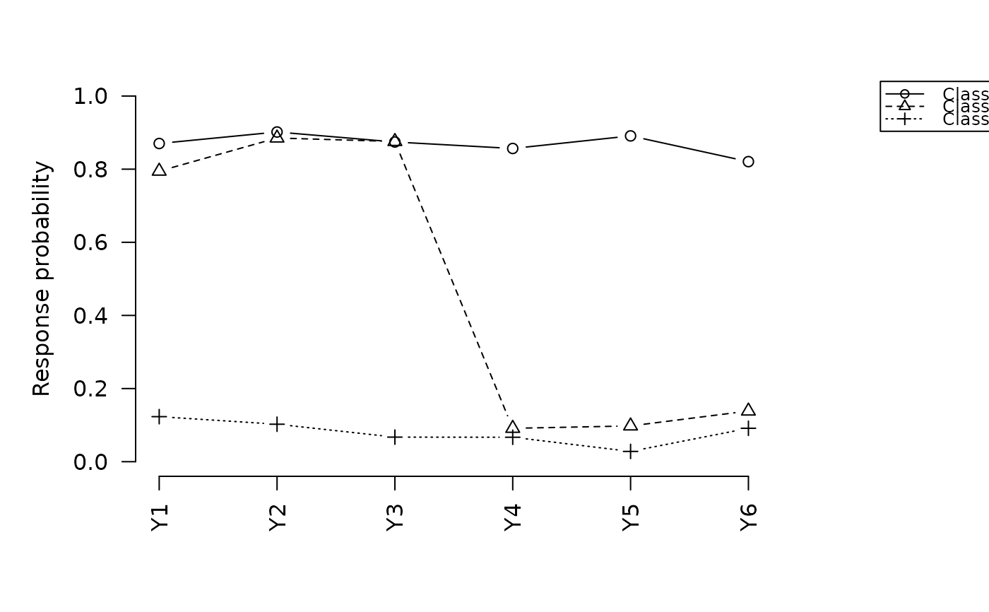
#> Item-response probabilities:
#>             C1      C2      C3
#> P(Y1|C) 0.8702 0.79457 0.12318
#> P(Y2|C) 0.9017 0.88526 0.10248
#> P(Y3|C) 0.8743 0.87570 0.06720
#> P(Y4|C) 0.8566 0.09128 0.06686
#> P(Y5|C) 0.8910 0.09781 0.02808
#> P(Y6|C) 0.8206 0.13853 0.09135

# ML three-step with simple SEs (fast)
fit <- three_step(d, Y.names = paste0("Y", 1:6), n_classes = 3,
                  Zp.names = "Zp", use.simple.cov = TRUE)
summary(fit)
#> Three-step latent class model: covariates
#>   Classes: 3   Estimator: ML   N: 200
#>   Log-lik: -548.6403 (df = 22)   AIC: 1141.28   BIC: 1213.84
#>   Entropy R² (covariate-adjusted): 0.8589
#> 
#> Covariate effects on class membership (multinomial logit):
#>                Estimate Std. Error z value Pr(>|z|)    
#> (Intercept):C2   2.2334     0.6258   3.569 0.000359 ***
#> Zp:C2           -1.1570     0.3002  -3.854 0.000116 ***
#> (Intercept):C3  -3.2742     0.7191  -4.553 5.29e-06 ***
#> Zp:C3            0.9401     0.1896   4.959 7.10e-07 ***
#> ---
#> Signif. codes:  0 ‘***’ 0.001 ‘**’ 0.01 ‘*’ 0.05 ‘.’ 0.1 ‘ ’ 1
coef(fit)
#> (Intercept):C2          Zp:C2 (Intercept):C3          Zp:C3 
#>      2.2333837     -1.1569878     -3.2742157      0.9400712 
vcov(fit)
#>                (Intercept):C2        Zp:C2 (Intercept):C3        Zp:C3
#> (Intercept):C2    0.391644881 -0.173583653    0.001643327 -0.002599746
#> Zp:C2            -0.173583653  0.090099886    0.016315352 -0.002300251
#> (Intercept):C3    0.001643327  0.016315352    0.517169347 -0.130664301
#> Zp:C3            -0.002599746 -0.002300251   -0.130664301  0.035941355

# Full measurement-uncertainty correction (see vignette for interpretation)
fit_cor <- three_step(d, Y.names = paste0("Y", 1:6), n_classes = 3,
                      Zp.names = "Zp", use.simple.cov = FALSE,
                      use.modal.assignment = FALSE)
summary(fit_cor)
#> Three-step latent class model: covariates
#>   Classes: 3   Estimator: ML   N: 200
#>   Log-lik: -548.4895 (df = 22)   AIC: 1140.98   BIC: 1213.54
#>   Entropy R² (covariate-adjusted): 0.8596
#> 
#> Covariate effects on class membership (multinomial logit):
#>                Estimate Std. Error z value Pr(>|z|)    
#> (Intercept):C2   2.0352     0.6182   3.292 0.000994 ***
#> Zp:C2           -1.0576     0.2974  -3.556 0.000377 ***
#> (Intercept):C3  -3.1385     0.6919  -4.536 5.74e-06 ***
#> Zp:C3            0.9090     0.1832   4.962 6.99e-07 ***
#> ---
#> Signif. codes:  0 ‘***’ 0.001 ‘**’ 0.01 ‘*’ 0.05 ‘.’ 0.1 ‘ ’ 1

# BCH estimator
fit_bch <- three_step(d, Y.names = paste0("Y", 1:6), n_classes = 3,
                      Zp.names = "Zp", use.bch = TRUE,
                      use.simple.cov = TRUE)
summary(fit_bch)
#> Three-step latent class model: covariates
#>   Classes: 3   Estimator: BCH   N: 200
#>   Log-lik: -548.5643 (df = 22)   AIC: 1141.13   BIC: 1213.69
#>   Entropy R² (covariate-adjusted): 0.8590
#> 
#> Covariate effects on class membership (multinomial logit):
#>                Estimate Std. Error z value Pr(>|z|)    
#> (Intercept):C2   2.1318     0.6582   3.239  0.00120 ** 
#> Zp:C2           -1.0967     0.3355  -3.269  0.00108 ** 
#> (Intercept):C3  -3.2851     0.8029  -4.091 4.29e-05 ***
#> Zp:C3            0.9407     0.2081   4.520 6.20e-06 ***
#> ---
#> Signif. codes:  0 ‘***’ 0.001 ‘**’ 0.01 ‘*’ 0.05 ‘.’ 0.1 ‘ ’ 1

# Change reference class
fit_c2 <- three_step(d, Y.names = paste0("Y", 1:6), n_classes = 3,
                     Zp.names = "Zp", use.simple.cov = TRUE,
                     rebase = "C2")
summary(fit_c2)
#> Three-step latent class model: covariates
#>   Classes: 3   Estimator: ML   N: 200
#>   Log-lik: -548.6403 (df = 22)   AIC: 1141.28   BIC: 1213.84
#>   Entropy R² (covariate-adjusted): 0.8589
#> 
#> Covariate effects on class membership (multinomial logit):
#>                Estimate Std. Error z value Pr(>|z|)    
#> (Intercept):C1  -2.2334     0.6258  -3.569 0.000359 ***
#> Zp:C1            1.1570     0.3002   3.854 0.000116 ***
#> (Intercept):C3  -5.5076     0.9516  -5.788 7.13e-09 ***
#> Zp:C3            2.0971     0.3614   5.802 6.56e-09 ***
#> ---
#> Signif. codes:  0 ‘***’ 0.001 ‘**’ 0.01 ‘*’ 0.05 ‘.’ 0.1 ‘ ’ 1

# Gaussian distal outcome
d2 <- generate_data(200, "high", "distal", seed = 2)
fit_dis <- three_step(d2, Y.names = paste0("Y", 1:6), n_classes = 3,
                      Zo.name = "Zo", family = "gaussian",
                      use.simple.cov = TRUE)
summary(fit_dis)
#> Three-step latent class model: distal outcome
#>   Classes: 3   Estimator: ML   Family: gaussian   N: 200
#>   Log-lik: -892.6754 (df = 24)   AIC: 1833.35   BIC: 1912.51
#> 
#> Distal outcome means by class:
#>       Estimate Std. Error z value Pr(>|z|)    
#> mu_C1 -0.82982    0.11555  -7.182 6.89e-13 ***
#> mu_C2  1.10449    0.11459   9.639  < 2e-16 ***
#> mu_C3  0.04204    0.15518   0.271    0.786    
#> ---
#> Signif. codes:  0 ‘***’ 0.001 ‘**’ 0.01 ‘*’ 0.05 ‘.’ 0.1 ‘ ’ 1

# Nominal categorical distal outcome (3+ categories): coef() returns a
# T x C matrix of class-conditional category probabilities; omnibus_test()
# gives a single Wald test of whether the category distribution differs
# across classes at all.
d2$Zcat <- factor(sample(c("low", "mid", "high"), nrow(d2), replace = TRUE))
fit_cat <- three_step(d2, Y.names = paste0("Y", 1:6), n_classes = 3,
                      Zo.name = "Zcat", family = "multinomial",
                      use.simple.cov = TRUE)
coef(fit_cat)
#>   C1:high   C2:high   C3:high    C1:low    C2:low    C3:low    C1:mid    C2:mid 
#> 0.2973475 0.4450948 0.3628017 0.3543067 0.2178582 0.2689451 0.3483458 0.3370470 
#>    C3:mid 
#> 0.3682532 
omnibus_test(fit_cat)
#> 
#> 	Wald test of equal distal outcome distributions across latent classes
#> 
#> data:  multinomial distal outcome, 3 classes
#> W = 3.6188, df = 4, p-value = 0.46
#> 

# Pass a pre-fitted measurement model to skip Step 1
fit_step1 <- three_step(d, Y.names = paste0("Y", 1:6), n_classes = 3)
fit2 <- three_step(d, Y.names = paste0("Y", 1:6), n_classes = 3,
                   Zp.names = "Zp", step1 = fit_step1,
                   use.simple.cov = TRUE)
summary(fit2)
#> Three-step latent class model: covariates
#>   Classes: 3   Estimator: ML   N: 200
#>   Log-lik: -548.6403 (df = 22)   AIC: 1141.28   BIC: 1213.84
#>   Entropy R² (covariate-adjusted): 0.8589
#> 
#> Covariate effects on class membership (multinomial logit):
#>                Estimate Std. Error z value Pr(>|z|)    
#> (Intercept):C2   2.2334     0.6258   3.569 0.000359 ***
#> Zp:C2           -1.1570     0.3002  -3.854 0.000116 ***
#> (Intercept):C3  -3.2742     0.7191  -4.553 5.29e-06 ***
#> Zp:C3            0.9401     0.1896   4.959 7.10e-07 ***
#> ---
#> Signif. codes:  0 ‘***’ 0.001 ‘**’ 0.01 ‘*’ 0.05 ‘.’ 0.1 ‘ ’ 1

# Supply an external starting classification for Step 1 (bypasses
# multilevLCA's k-means-on-PCA initialization; here we use the DGP's own
# true classes as a stand-in for e.g. a StepMix solution with many
# random starts)
fit_ext <- three_step(d, Y.names = paste0("Y", 1:6), n_classes = 3,
                      startval = d$X, use.simple.cov = TRUE)
summary(fit_ext)
#> Latent class measurement model
#>   Classes: 3   N: 200
#>   Log-lik: -595.2880 (df = 20)   AIC: 1230.58   BIC: 1296.54
#>   Entropy R²: 0.8430
#> 
#> Class sizes:
#>     C1     C2     C3 
#> 0.3495 0.2915 0.3590 
#> 
#> Item-response probabilities:
#>             C1      C2      C3
#> P(Y1|C) 0.8702 0.79457 0.12318
#> P(Y2|C) 0.9017 0.88525 0.10248
#> P(Y3|C) 0.8743 0.87570 0.06720
#> P(Y4|C) 0.8566 0.09128 0.06686
#> P(Y5|C) 0.8910 0.09781 0.02808
#> P(Y6|C) 0.8206 0.13853 0.09135

# Many random-classification restarts for Step 1, keeping the best
# (analogous to n_init in StepMix or nrep in poLCA)
fit_ninit <- three_step(d, Y.names = paste0("Y", 1:6), n_classes = 3,
                        n_init = 20L, use.simple.cov = TRUE)
summary(fit_ninit)
#> Latent class measurement model
#>   Classes: 3   N: 200
#>   Log-lik: -595.2880 (df = 20)   AIC: 1230.58   BIC: 1296.54
#>   Entropy R²: 0.8430
#> 
#> Class sizes:
#>     C1     C2     C3 
#> 0.3495 0.2915 0.3590 
#> 
#> Item-response probabilities:
#>             C1      C2      C3
#> P(Y1|C) 0.8702 0.79456 0.12317
#> P(Y2|C) 0.9017 0.88524 0.10247
#> P(Y3|C) 0.8743 0.87569 0.06719
#> P(Y4|C) 0.8566 0.09127 0.06686
#> P(Y5|C) 0.8910 0.09780 0.02808
#> P(Y6|C) 0.8206 0.13853 0.09135

# Plot item-response profiles from the measurement model
plot(fit)