This project is part of a two-post series. See the first post here
All code and progress for this project is kept up to date at https://github.com/SamLeeBYU/BYUTrafficCitations.
Introduction
Both private and public universities across the United Sates typically have university-specific parking service to enforce university parking regulations due to limited parking space supply. For the purposes of this analysis, we will analyze traffic citation data specific to my university, Brigham Young University.
The purpose behind this analysis will be to see if we can trace out any signal behind the relationship of number of traffic citations given on a particular day and effects in weather and air quality. We hypothesize that when adjusted for confounding effects such as changes in enrollment, seasonality, type of day (whether the day is a holiday), day of week, and trends in time, we can isolate the effect of all influential factors that affect trends in traffic citations given at BYU.
We hypothesize that changes in weather patterns change the incentives of students’ choices in transportation choice as well as incentives for BYU’s parking enforcement task force. We make the assumption that incentives for students’ choices in transportation are more inelastic in regards to changes in weather as opposed to incentives for BYU’s parking enforcement task force.
If this theory holds then through regression analysis, we hope to show that increase in negative weather effects will significantly decrease the amount of traffic citations distributed on a particular day.
If incentives for students’ choices in transportation are indeed more inelastic than the incentives for parking police at BYU with respect to changes in weather and air quality, then this provides convincing evidence that as trends in weather and air quality become more severe, weather factors become a greater indicator of changes in parking demand than parking citations.
As stated last time, I want to know if changes in the number of traffic citations from day to day or week to week depends on the incentives of students’ transportation choices in the midst of weather and air quality effects. On the contrary, are the small fluctuations in the number of traffic citations from day to day and week to week just simply due to random error or something else that’s not captured in the data?
Exploratory Data Analysis
Through exploratory data analysis we hope to answer the following questions with our data set:
- Does the daily number of traffic fines depend on the day of the week?
- Can we dispel or prove the common rumor that parking police have “quotas”?
- How does AQI affect changes in the daily number of fines?
- Is there any strong multicollinearity between any of the weather factors?
- Can we predict the daily number of fines over a certain span of time?
Explore the documented EDA process in EDA.ipynb.
Does the daily number of traffic fines depend on the day of the week?
In order to model short-run changes in the daily number of fines, controlling for the day of the week would seem natural. Hypothetically, students could be inherently more likely to come school anyways on certain days regardless of what parking police do and regardless of the weather.
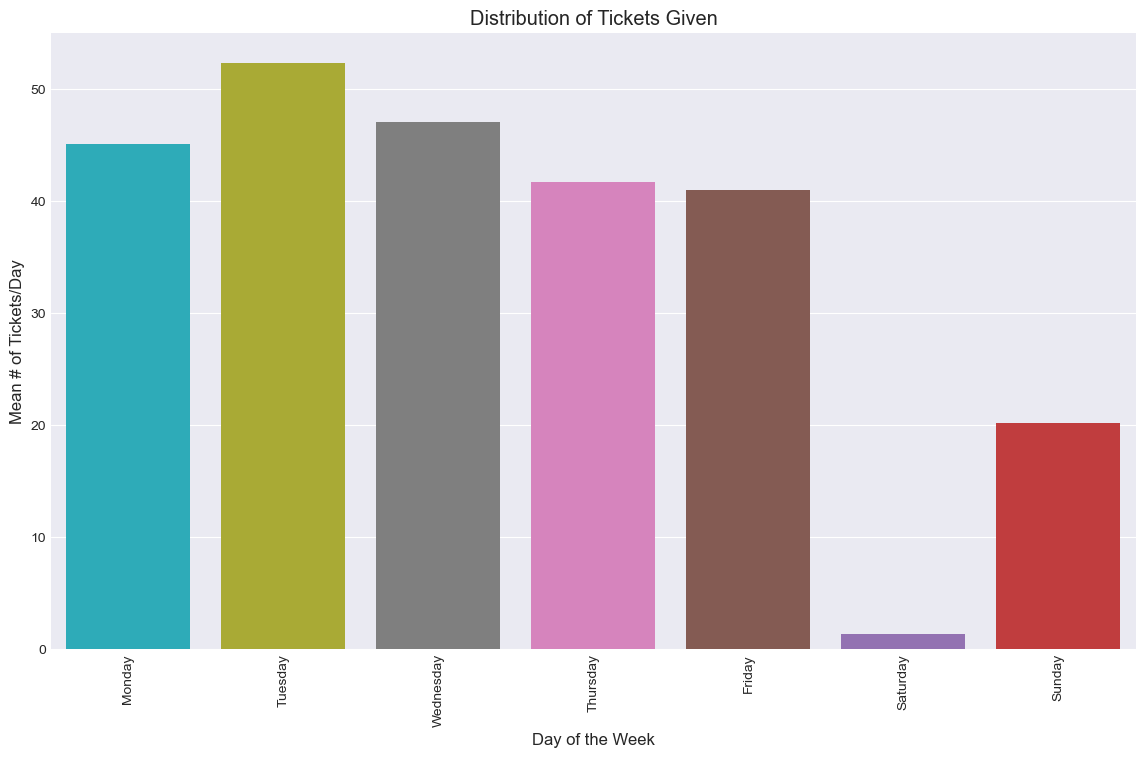
Not a surprise, this shows that Saturday had lowest mean number of tickets given per day out of all days of the week–this could be due to the fact that parking rules are drastically relaxed on Saturday in addition to there being a lower demand in students. We assume that on average, the parking police don’t change their strategies depending on the day of the week.
What’s more interesting is when we look at the lag plot for the daily number of fines:
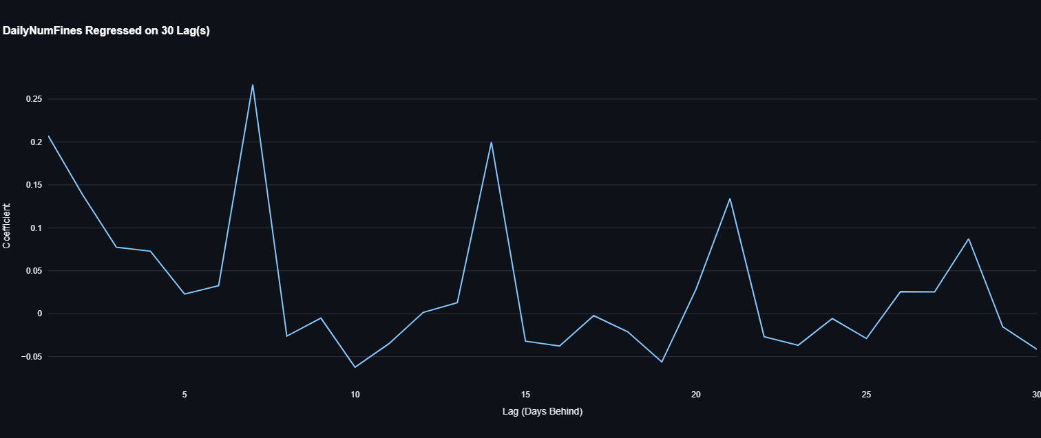
A lag variable is just the response variable but from the past. A pth lag is $Y_{t-p}$, where p is the time interval and $Y_t$ is the response variable for each period $t$. For those who haven’t seen lag variables before it might seem weird to form a regression such that $Y_t=\beta_0+\beta_pY_{t-p}+\epsilon_t$, but that’s exactly what we’re doing. The graph you see above is a graph of the coefficients, $p$. We normally use lag variables when we suspect we have highly dependent data. We usually expect that as $p$ increases the coefficient $\beta_p$ shrinks to zero. In other words, the response from $p$ time periods ago becomes less of a good metric to predict the response variable right now (at time $t$).
What we see here is really interesting in regards to this question. The coefficients peak at exactly 7, 14, 21, and 28. These are multiples of 7. This implies that the daily number of fines are dependent about the daily number of fines from one week, two weeks, three weeks ago, and four weeks ago more so than it is than, say two days ago. This may be evidence that the parking police have a weekly quota, but we will see in the next question why this is nuanced. This is most likely due to the fact that every Saturday parking demand drastically falls and parking rules become much more lax.
Can we dispel or prove the common rumor that parking police have “quotas”?
Due to shared frustration among students at any university with strict allocation of resources, including parking resources, it becomes a popular discussion from time to time to figure out why the parking police seem to distribute so many citations. Some students figure that the parking must have certain quotas to meet. This could be a reasonable theory. Afterall, in 2022 alone, BYU parking police collected a total of $705,836 in paid fines. Granted, a fraction of these come from non-BYU students. I’ll leave that up to you to figure out whether that’s a reasonable amount.
The data, however, tend to refute the hypothesis that there’s a general quota:
#Can we show that parking services have a quota?

Provo["DayNum"] = Provo["DATE"].dt.day

bi_weekly_tickets = []
monthly_tickets = []
total = 0
monthly_total = 0
month = ""
for i, row in Provo.iterrows():
    if row["Day"] == "Saturday" and i % 2 == 0:
        bi_weekly_tickets.append(total)
        total = 0
    if row["Month"] != month:
        monthly_tickets.append(total)
        monthly_total = 0
        month = row["Month"]
    total += row["DailyNumFines"]
    monthly_total += row["DailyNumFines"]

plt.hist(bi_weekly_tickets, bins=30, color='skyblue', edgecolor='black')

plt.xlabel('Number of Tickets')
plt.ylabel('Frequency')
plt.title('Histogram of an Bi-Weekly Cumulative Number of Tickets')

plt.show()
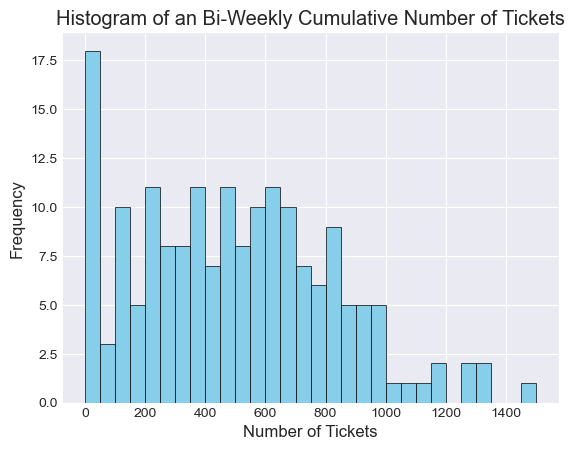
Defining a complete week as Saturday to Saturday, we can look at the bi-weekly distribution number of tickets. If there was a quota, or a bi-weekly quota, we would expect this distribution to center on a value, or at the very least, exhibit low variance, but we don’t see this in the data. It is possible that quotas (if such a thing exists), are more sophisticated and they are differentiate across different officers or different types of tickets (i.e. different price of fines); or perhaps they vary across month and season. This could explain the non-conformity and large variance we see in the distribution we see above.
We could look at monthly quotas as well…
plt.hist(monthly_tickets, bins=12*9-5, color='firebrick', edgecolor='black', alpha=0.5)
plt.hist(monthly_tickets, bins=12*9-5, color='firebrick', edgecolor='black', alpha=0.5)
plt.xlabel('Number of Tickets')
plt.ylabel('Frequency')
plt.title('Histogram of an Monthly Cumulative Number of Tickets')

plt.show()
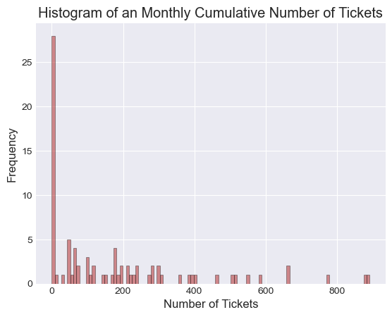
The case for a monthly quota is even worse, as there is a larger variance.
Based on preliminary data analysis, it doesn’t appear there to be a general quota. This is beneficial for the research question as whole: If we expected quotas, and parking services had no incentives to change how many fines they distributed on a particular day, then we wouldn’t be able to infer much about students changed their choices as well.
How does AQI affect changes in the daily number of fines?
Now that we eliminated potential confounders in the distribution of the daily number of fines, we can start analyzing the direct effect that air quality has the number of daily fines. Air Quality Index (AQI) is a proportional calculation of whatever pollutant is the most extreme for that given time period [4]. We hypothesize that worse air quality will decrease the number of traffic fines distributed for 1 or 2 reasons:
- If the air quality becomes worse enough, even for students who drive to campus, since walking around campus is a necessity, it could change the incentive for these risk adverse individuals so much to the extent that coming to school at all may not be worth it. Other economic studies have shown that poor air quality has decreased school attendance so while this theory may be marginal for students in Provo, where the AQI doesn’t typically exceed unhealthy levels, there could still exist some signal within this. Since AQI may be correlated with other weather factors such as rain, snow, PM10, changes in AQI while may not directly affect number of daily fines could signal to other weather effects that do.
- Either AQI or correlated factors with AQI change the incentives of parking police such that it is either marginally too difficult to distribute parking citations during these periods, or the resulting weather conditions make it impractical to cite vehicles: For example, it would be unlikely for parking police to cite someone during a severe thunderstorm even if they were breaking policy.
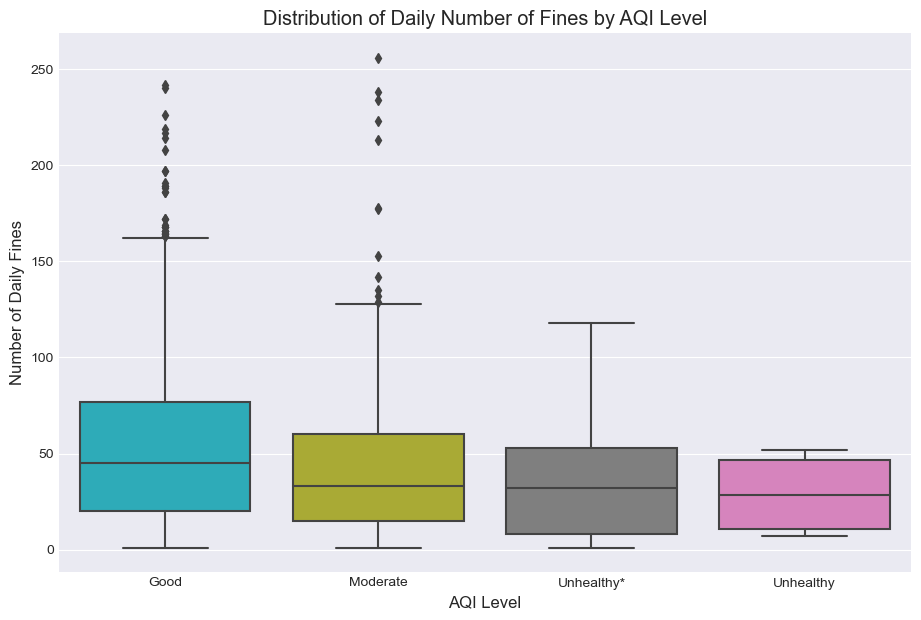
The boxplot distributions imply a general negative association between AQI and the daily number of fines given, as hypothesized. However, the signal is weak if anything. We will need to adjust for covariates to interpret this effect.
Upon closer inspection of these trends, we can examine how AQI compare against the daily number of fines for a specific month. In EDA.ipynb I have it sample random months to see if there is a general trend. Here is one plot–the minimum temperature is also thrown in there as a control against AQI and changes in number of fines.
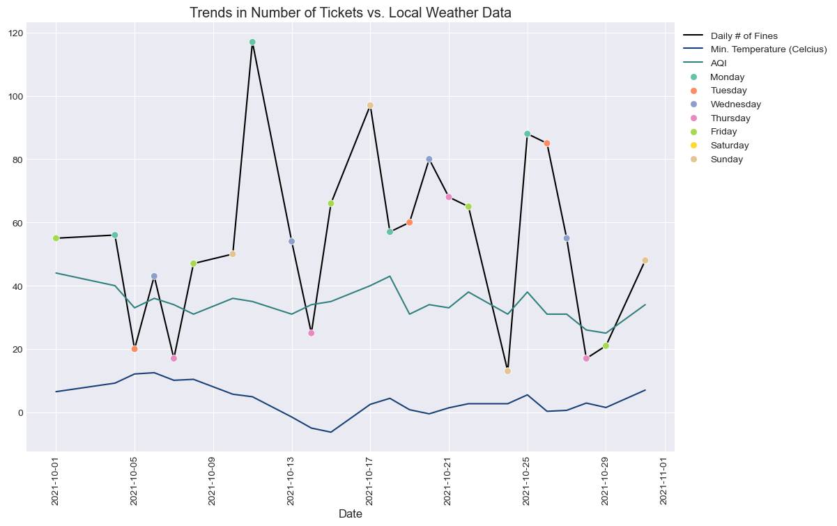
The data are extremely noisy. It is still possible that students on the margin are influenced by weather and air quality factors, but without regression analysis, we cannot determine a specific effect for AQI.
Is there any strong multicollinearity between any of the weather factors?
As mentioned in earlier sections, there may be strong colinearity between the weather factors and air quality factors. In regression analysis this could inflate the variance of the estimators. I looked at a heatmap of the correlations between all the weather and environmental factors.
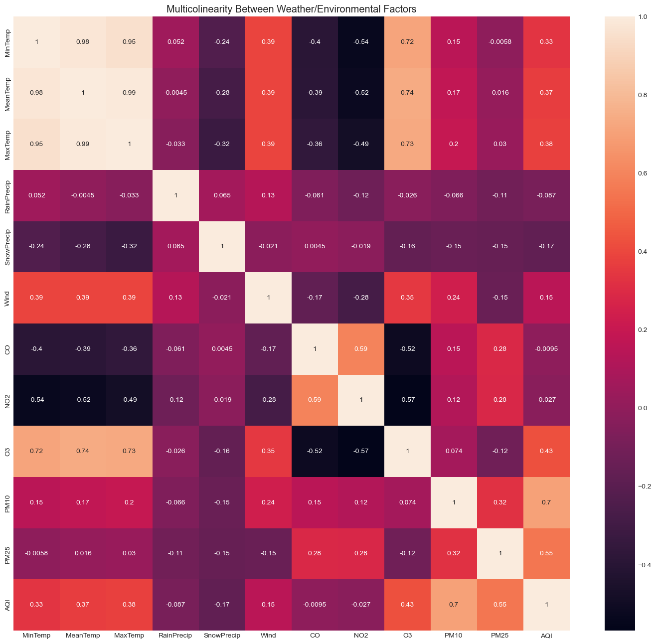
All the temperature factors are basically a perfect match. This isn’t surprising. The pollutants $CO$, $NO_2$, and $O_3$ appear to have strong relations with temperature, although perhaps the only one with a strong colinearity is $O_3$.
The most interesting factor to look at in this matrix is AQI. It is most strongly correlated with the particulate matter factors, PM10 and PM2.5. This implies that PM10 and PM2.5 are typically the worse pollutants–or the most assailant pollutants in the atmosphere.
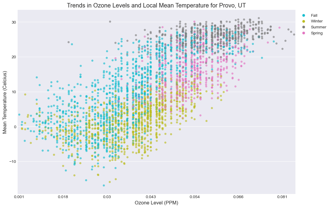
Upon looking further into the relationship of $O_3$ and temperature, it appears that $O_3$ varies between seasons:
Can we predict the daily number of fines over a certain span of time?
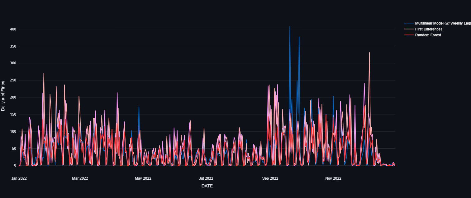
We are finally ready to use our data set to make inferential predictions about the daily number of fines with the goal being to isolate the effect of signal of the environmental factors. I will cover the statistical details in a future blog post, but I created three models: A multilinear regression model with weekly lags (weekly lags corresponding to $DailyNumFines_{t-1}$, $DailyNumFines_{t-7}$, $DailyNumFines_{t-14}$, $DailyNumFines_{t-21}$, $DailyNumFines_{t-28}$), a first differences model, and a random forest model for prediction. For the purposes of modeling, I modeled the log number of daily number of fines.
I put all models on display on this project’s dashboard.
Here is the graphical output for the year 2022:
Or by taking a rolling average of 30 days to adjust the smoothness of the graph,
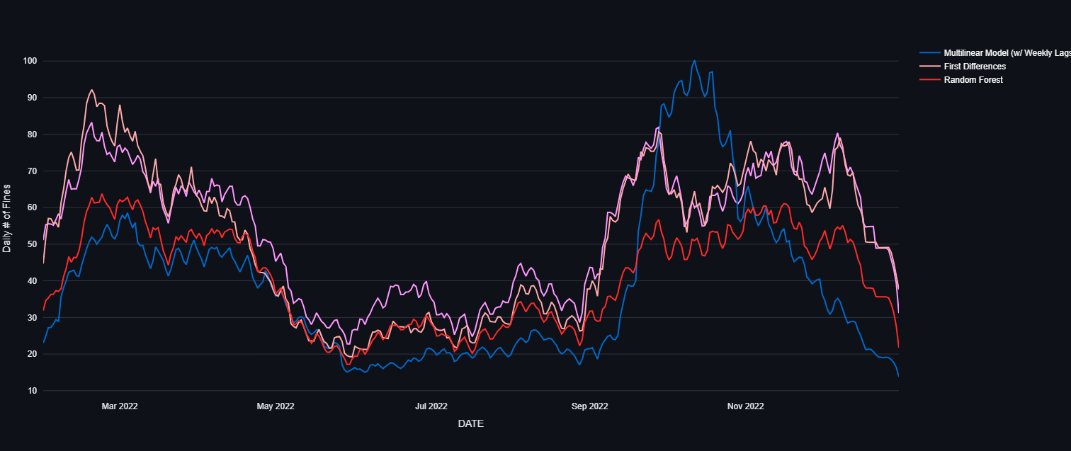
The random forest takes consistently overestimates whereas in place of accuracy, the multilinear model averages around the true mean. The first differences model is the best approximation to model the daily number of fines just by looking at year 2022.
Our first difference model yielded significant p-values for the following environmental factors (controlling for other effects):
| Variable | Estimate | Std. Error | t-value | p-value |
|---|---|---|---|---|
| $\Delta \text{NO}_{2t}\times \Delta \text{PM10}_t$ | -0.000368 | 0.0000819 | -4.493 | 0.00000736 |
| $\Delta \text{MaxTemp}_t \times I(\text{Season}_t = \text{Summer})$ | 0.04114 | 0.02227 | 1.847 | 0.064905 |
| $\Delta \text{AQI}_t \times I(\text{Month}_t = \text{February}_t)$ | -0.01552 | 0.006942 | -2.236 | 0.025442 |
| $\Delta \text{CO}_{3t} \times I(\text{Season}_t = \text{Spring})$ | 1.86 | 0.9924 | 1.874 | 0.061047 |
| $\Delta \text{RainPrecip}_t \times I(\text{Month}_t = \text{December})$ | -0.5382 | 0.2228 | -2.416 | 0.015779 |
As hypothesized, the coefficient for $\Delta AQI\times I(Month_t=February)$ is significantly negative, although specifically for months of February. This means for days in February, all else in constant, we would expect the daily change in the log number of fines to decrease by -0.1552 for every increase in the AQI.
Concluding Statement
In this exploratory data analysis project we sought out signal in a noisy data set. While the daily number of traffic citations has a distinctive seasonal pattern, the short-run patterns are more or less random. Nevertheless, we conjecture that controlling for all other fixed and lagged effects, that there are some significant environmental and weather predictors. This preliminary analysis is sufficient to indicate that there may be signal for these effects: Indeed, changes in environmental factors may alter students’ incentives to come to class on the margin. It may also alter the incentive for parking police to distribute tickets. This needs to be investigated further, probably in a city or region that has more severe and more variable air pollutant climate than Provo, UT.